Visualizing canonical markers and spatially variable genes in Visium data

1. What data types are you visualizing?
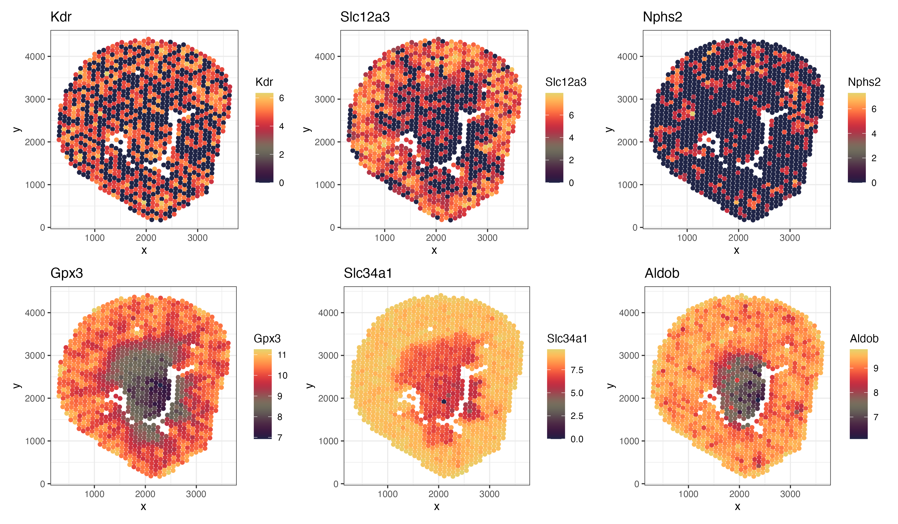
I’m visualizing quantitative gene expression values for multiple genes across quantitative spatial coordinates (x, y) for each visium spot. The gene expression values I plot are normalized and log-transformed.
2. What data encodings (geometric primitives and visual channels) are you using to visualize these data types?
I use points as the geometric primitive. As for visual channel, I use x-axis and y-axis position to encode location for each spot and use hue intensity to encode the continuous expression level of the gene.
3. What about the data are you trying to make salient through this data visualization?
I’m trying to make salient where spots show high expression of canonical markers such as Slc12a3 and Kdr (Park et al., 2018) and where top spatially variable genes show patterns.
Jihwan Park et al. ,Single-cell transcriptomics of the mouse kidney reveals potential cellular targets of kidney disease.Science360,758-763(2018).DOI:10.1126/science.aar2131
4. What Gestalt principles or knowledge about perceptiveness of visual encodings are you using to accomplish this?
I mainly used the Gestalt principle of similarity that spots with similar colors are perceived as grouped and related, so regions with similar expression levels would stand out.
5. Code
1
2
3
4
5
6
7
8
9
10
11
12
13
14
15
16
17
18
19
20
21
22
23
24
25
26
27
28
29
30
31
32
33
34
35
36
37
38
39
40
41
42
43
44
45
46
47
48
49
50
51
52
53
54
55
56
57
58
59
60
61
62
63
64
65
66
67
68
69
70
71
72
73
74
75
76
77
78
79
80
#data visualization
#HW1

library(dplyr)
library(ggplot2)
library(gridExtra)
library(jcolors)
library(Seurat)
library(patchwork)
library(tidyverse)

setwd("/Users/tiya/Desktop/BME\ program\ info/Spring\ 2026/gemonic_data_visal")

dat = read_csv("data/Visium-IRI-ShamR_matrix.csv")
dim(dat) #[1]  1224 19468

#change cell name
colnames(dat)[1] = "spot"
genes = colnames(dat)[-c(1, 2, 3)]

#normalize the data
table(dat[, 5])
table(dat[, ncol(dat)/4])
table(dat[, ncol(dat)/2])#even though there is no description, from the integer distribution of gene counts, it appears that the data are not normalized

total_counts_spot <- rowSums(dat[, genes])
all(total_counts_spot > 0) #[1] TRUE
all(!is.na(total_counts_spot)) #[1] TRUE

normalized_genes = matrix()
for(i in 1:length(genes)){
  normalized_gene = log1p((dat[, genes[i]] / total_counts_spot)*1e6)
  normalized_genes = cbind(normalized_genes, normalized_gene)
}

normalized_genes = cbind(dat %>% select(spot, x, y),
                         normalized_genes %>% select(-normalized_genes))
dim(normalized_genes) == dim(dat)

rownames(normalized_genes) = normalized_genes$spot

#some canonical marker genes from paper "Single-cell transcriptomics of the mouse kidney reveals potential cellular targets of kidney disease" by Park et al., on 2018
#https://www.science.org/doi/10.1126/science.aar2131
#Some of the examples they listed are "Kdr (encoding vascular endothelial growth factor receptor 2) for endothelial cells", "Slc12a3 (thiazide-sensitive sodium chloride cotransporter) for the distal convoluted tubule", and "Nphs2 (podocin) for podocytes".

plot_gene = function(gene_of_interest){

  ggplot(normalized_genes, aes(x = x, y = y, color = get(gene_of_interest))) +
    geom_point() +
    theme_bw() +
    scale_color_jcolors_contin("pal4") +
    ggtitle(gene_of_interest) +
    labs(color = gene_of_interest)
}

p1 = plot_gene("Kdr")
p2 = plot_gene("Slc12a3")
p3 = plot_gene("Nphs2")

#pick some spacially variable genes across spots
normalized_genes_matrix = normalized_genes
normalized_genes_matrix = normalized_genes[, genes] %>% as.matrix()
outs = FindSpatiallyVariableFeatures(
  object = t(normalized_genes_matrix),
  spatial.location = as.matrix(normalized_genes[, c("x", "y")]),
  selection.method = "moransi",
  verbose = FALSE
)
# Top spatial genes
outs_top <- outs[order(outs$p.value, -outs$observed), ]
head(outs_top, 3) #Gpx3, Slc34a1, Aldob

p4 = plot_gene("Gpx3")
p5 = plot_gene("Slc34a1")
p6 = plot_gene("Aldob")

(p1+p2+p3)/(p4+p5+p6)
ggsave("hw/hw1_tzhan104.png", width = 12, height = 7)