Visualizing Spatial Gene Expression with PCA and tSNE

1. How do the gene loadings on the first PC relate to features of the genes such as its mean or variance?
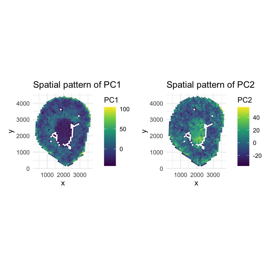
The first principal component captures the direction of maximal variance in the gene expression data. Genes with large absolute loadings on PC1 are those that contribute most strongly to this variance, meaning they exhibit substantial variation across spatial spots. In the PC1 spatial plot, this is reflected by regions with high and low PC scores, which correspond to spots where these high-loading genes are differentially expressed.
Importantly, PC1 loadings are more closely related to a gene’s variance than to its mean expression level. Genes that have high mean expression but are relatively uniform across the tissue tend to have small loadings because they do not drive differences between spots. In contrast, genes with high spatial variability contribute strongly to PC1 and shape the spatial patterns observed in the plot. Thus, the PC1 visualization highlights spatial structure driven by high-variance genes rather than overall expression magnitude.
5. Code (paste your code in between the ``` symbols)
1
2
3
4
5
6
7
8
9
10
11
12
13
14
15
16
17
18
19
20
21
22
23
24
25
26
27
28
29
30
31
32
33
34
35
36
37
38
39
40
41
42
43
44
45
46
library(ggplot2)

# ---- Load data ----
data <- read.csv("~/Desktop/Visium-IRI-ShamR_matrix.csv.gz")

# ---- Spatial coordinates ----
pos <- data[, c("x", "y")]

# ---- Gene expression ----
gexp <- data[, sapply(data, is.numeric)]
gexp <- gexp[, !(colnames(gexp) %in% c("x", "y"))]

# ---- Remove constant/zero-variance genes ----
keep_var <- apply(gexp, 2, sd, na.rm = TRUE) > 0
gexp <- gexp[, keep_var]


# ---- PCA  ----
pca <- prcomp(gexp, center = TRUE, scale. = TRUE)

# ---- Data for plotting ----
df <- data.frame(
  x = pos$x,
  y = pos$y,
  PC1 = pca$x[, 1],
  PC2 = pca$x[, 2]
)

# ---- 2-panel spatial PCA visualization ----
p1 <- ggplot(df, aes(x, y, color = PC1)) +
  geom_point(size = 0.5) +
  scale_color_viridis_c() +
  coord_fixed() +
  theme_minimal() +
  labs(title = "Spatial pattern of PC1")

p2 <- ggplot(df, aes(x, y, color = PC2)) +
  geom_point(size = 0.5) +
  scale_color_viridis_c() +
  coord_fixed() +
  theme_minimal() +
  labs(title = "Spatial pattern of PC2")

library(patchwork)
p1 + p2