HW2 Submission

2. How do the genes with high versus low loadings relate to each other? How are they patterned relative to each other in the tissue?
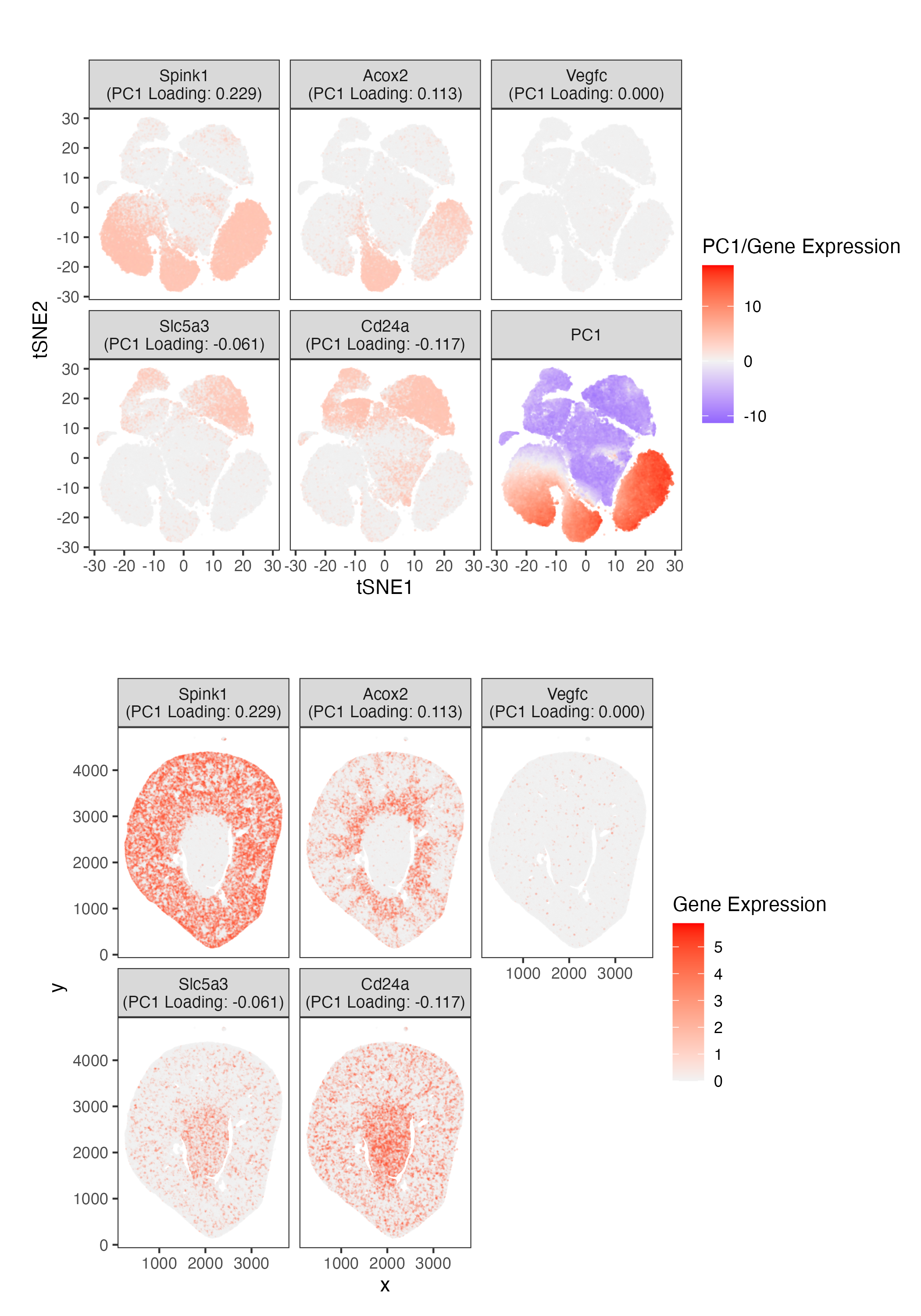
Genes with high loadings on a principal component (PC) in principal component analysis (PCA) are the highly expressed drivers of the PC axis, and are often co-expressed when the loading is positive. This is shown by the expression of the Spink1 gene (highest loading on PC1: 0.229) and the Acox2 gene (moderately high loading on PC1: 0.113) being upregulated in similar tSNE coordinates/cells as where the PC1 score is increased, indicating that the genes with high loading drive the dominant source of variation captured by PC1. Conversely, genes with low loadings on a PC in PCA are the highly expressed non-drivers of the PC axis, and are often co-expressed when the loading is negative. This is shown by the expression of the Cd24a gene (lowest loading on PC1: -0.117) and the Slc5a3 gene (moderately low loading on PC1: -0.061) being upregulated in similar tSNE coordinates/cells as where PC1 score is decreased, indicating that the genes with low loading oppose the dominant source of variation captured by PC1. Additionally, genes with near-zero loadings on a PC in PCA are neither drivers nor non-drivers of the PC axis, and are consistently minimally expressed when the loading is positive, near-zero, or negative. This is shown by the expression of the Vegfc gene (near-zero loading on PC1: 0.000) being neither upregulated nor downregulated in any of the tSNE coordinates/cells, regardless of whether the PC1 score is high, near-zero, or low, indicating that the genes with near-zero loading do not drive or oppose the dominant source of variation captured by PC1. Genes with high loadings (e.g., Spink1, highest loading on PC1: 0.229; Acox2, moderately high loading on PC1: 0.113) and low loadings (e.g., Cd24a, lowest loading on PC1: -0.117; Slc5a3, moderately low loading on PC1: -0.061) on a PC in PCA are expressed on opposite spatial regions in the tissue. Genes with highest (e.g., Spink1) and moderately high (e.g., Acox2) loadings, as well as genes with lowest (e.g., Cd24a) and moderately low (e.g., Slc5a3) loadings, both differ in expression, as the former is more highly expressed than the latter for each pair, despite similar ubiquity and co-expression in comparable spatial regions of the same tissue. Genes with near-zero loadings (e.g., Vegfc, near-zero loading on PC1: 0.000) on a PC are minimally and ubiquitously expressed throughout spatial regions in the tissue. Given that spatial regions with similar gene expression suggest close transcriptional and biological activity, if the expressed genes are markers for certain cell types, there is a possibility that genes with high and low loadings in a tissue define separate particular cell types.
1. What data types are you visualizing?
I am visualizing quantitative data of the gene expression counts of multiple genes with different loadings on PC1 (Spink1, Acox2, Cd24a, Slc5a3, and Vegfc) for each cell, as well as quantitative data of the PC1 scores from PCA (linear dimensionality reduction) at a single-cell resolution. Additionally, I am visualizing spatial data of the x, y positions of the tissue, which helps relate the gene expression counts of multiple genes with different loadings on PC1 (Spink1, Acox2, Cd24a, Slc5a3, and Vegfc) to a spatial context in the same physical tissue.
2. What data encodings (geometric primitives and visual channels) are you using to visualize these data types?
I am using the geometric primitive of points to plot each cell. I am using the visual channels of position along the x-axis and position along the y-axis in two separate coordinate systems: tSNE1 and tSNE2, respectively, to show transcriptomic similarity and PC1 scores in a reduced space (top six panels), along with positional x and positional y, respectively, to demonstrate spatial context in the same physical tissue (bottom five panels). I am using the visual channel of hue, by going through blue to light grey to red, to encode the expression counts of the multiple genes with different loadings on PC1 (Spink1, Acox2, Cd24a, Slc5a3, and Vegfc) and PC1 scores (top six panels), as well as by going through light grey to red, to encode the expression counts of the above five genes (bottom five panels).
3. What about the data are you trying to make salient through this data visualization?
I am trying to make salient how genes with high versus low PC1 loadings relate to each other, transcriptionally and spatially. Genes with high loadings (Spink1, Acox2) on PC1 are the highly expressed drivers of the PC axis, and are often co-expressed when the loading is positive; conversely, genes with low loadings (Cd24a, Slc5a3) on PC1 are the highly expressed non-drivers of the PC axis, and are often co-expressed when the loading is negative. Furthermore, genes with near-zero loadings on PC1 (Vegfc) are neither drivers nor non-drivers of the PC axis, and are consistently minimally expressed when the loading is positive, near-zero, or negative. Genes with high loadings (Spink1, Acox2) and low loadings (Cd24a, Slc5a3) on PC1 are expressed on opposing, complementary spatial regions in the tissue. Genes with the highest (Spink1) and moderately high (Acox2) loadings, as well as genes with the lowest (Cd24a) and moderately low loadings (Slc5a3), both differ in expression, as the former is more highly expressed than the latter for each pair, despite similar ubiquity and co-expression in comparable spatial regions of the same tissue. Genes with near-zero loadings (Vegfc) on PC1 are minimally and ubiquitously expressed throughout spatial regions in the tissue.
4. What Gestalt principles or knowledge about perceptiveness of visual encodings are you using to accomplish this?
I am using the Gestalt principle of similarity, where items alike in their visual channels, specifically hue in this instance, tend to be perceived as being in a related group. By implementing color scales where similar gene expression counts/PC1 scores correspond to similar hues, I make salient the cells with similar gene expression or PC1 values. I am also using the Gestalt principle of proximity, where items that are near each other tend to be perceived as being a related group. By plotting points representing each cell, I make salient the nearby cluster of cells that have similar gene expressions/PC1 scores (top six panels and bottom five panels); moreover, I make salient the nearby clusters of cells that are located in spatially similar tissue regions (bottom five panels).
5. Code
1
2
3
4
5
6
7
8
9
10
11
12
13
14
15
16
17
18
19
20
21
22
23
24
25
26
27
28
29
30
31
32
33
34
35
36
37
38
39
40
41
42
43
44
45
46
47
48
49
50
51
52
53
54
55
56
57
58
59
60
61
62
63
64
65
66
67
68
69
70
71
72
73
74
75
76
77
78
79
80
81
# Load the necessary libraries
library(ggplot2)
library(tidyr)
library(dplyr)
library(patchwork)

# Read in data
data <- read.csv('~/Documents/genomic-data-visualization-2026/data/Xenium-IRI-ShamR_matrix.csv.gz')
pos <- data[,c('x', 'y')]
rownames(pos) <- data[,1]
gexp <- data[, 4:ncol(data)]
rownames(gexp) <- data[,1]

# Normalize
totgexp <- rowSums(gexp)
mat <- log10(gexp/totgexp * 1e6 + 1)

# PCA: linear dimensionality reduction
pcs <- prcomp(mat, center=TRUE, scale=FALSE)
sort(pcs$rotation[,1], decreasing=TRUE)

# tSNE: non-linear dimensionality reduction
toppcs <- pcs$x[, 1:10]
set.seed(20326)
tsne <- Rtsne::Rtsne(toppcs, dims=2, perplexity=30, verbose=TRUE)
emb <- tsne$Y
rownames(emb) <- rownames(mat)
colnames(emb) <- c('tSNE1', 'tSNE2')
head(emb)

# Genes to visualize: selected from the sorted list of genes in Line 20 above, since
# Spink1 has the highest loading, Vegfc has the loading closest to 0, Cd24a has the lowest loading,
# Acox2 has a moderately high loading around the midpoint of Spink1 and Vegfc, and
# Slc5a3 has a moderately low loading around the midpoint of Vegfc and Cd24a
genes <- c("Spink1", "Acox2", "Vegfc", "Slc5a3", "Cd24a")

# Build data frame with positional coordinates, PCs, and gene expression
df <- data.frame(pos, emb, pcs$x[, 1:10, drop = FALSE], mat[, genes, drop = FALSE])

# Set facet labels to display PC1 loading values
# Prompt to AI: "How do I place a loading number notation right under the plot title (gene) in paranthesis?"
load_PC1 <- pcs$rotation[genes, 1]
facet_labels <- c(setNames(paste0(genes, "\n(PC1 Loading: ", sprintf("%.3f", load_PC1), ")"), genes), PC1 = "PC1")

# Set long format for top plot (tSNE)
# Prompt to AI: "How do I make the order of display (from top left to bottom right) be: PC1, gene1, gene2, gene3, gene4, gene5?"
df_long_top <- df %>%
  pivot_longer(cols = c(all_of(genes), PC1), names_to = "feature", values_to = "value") %>%
  mutate(feature = factor(feature, levels = c(genes, "PC1")))

# Set long format for bottom plot (spatial)
# Adapted from the code above
df_long_bottom <- df %>%
  pivot_longer(cols = all_of(genes), names_to = "feature", values_to = "value") %>%
  mutate(feature = factor(feature, levels = genes))

# Top plot: tSNE
p_tsne <- ggplot(df_long_top, aes(tSNE1, tSNE2, col = value)) +
  geom_point(size = 0.01, alpha = 0.2) +
  facet_wrap(~feature, nrow = 2, ncol = 3, labeller = labeller(feature = facet_labels)) +
  scale_color_gradient2(low = "blue", mid = "grey95", high = "red") +
  theme_test() +
  theme(strip.text = element_text(size = 9), legend.position = "right") +
  coord_fixed() +
  labs(col = "PC1/Gene Expression")

# Bottom plot: spatial
# Prompt to AI: "How do I add another ggplot (nrow = 2, ncol = 3) physically under an existing ggplot (nrow = 2, ncol = 3)?"
p_bottom <- ggplot(df_long_bottom, aes(x, y, col = value)) +
  geom_point(size = 0.01, alpha = 0.2) +
  facet_wrap(~feature, nrow = 2, ncol = 3, labeller = labeller(feature = facet_labels)) +
  scale_color_gradient2(low = "blue", mid = "grey95", high = "red") +
  theme_test() +
  theme(strip.text = element_text(size = 9), legend.position = c(1.18,0.5)) +
  coord_fixed() +
  labs(col = "Gene Expression")

# Stack the top plot (tSNE) on the bottom plot (spatial) and save as a .png file
p_all <- (p_tsne / plot_spacer() / p_bottom) + plot_layout(heights = c(1, 0, 1))
p_all
ggsave("hw2_yhodo1.png", p_all, width = 7, height = 10, dpi = 300)