HW 2

1. How do the gene loadings on the first PC relate to features of the genes such as its mean or variance?
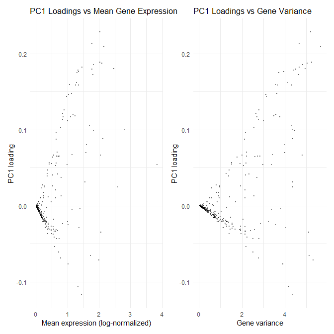
For context, the data was log-transformed, but not scaled, so genes with larger variance have more influence on the first PC. Genes with zero variance were also dropped because those genes cannot include PC1. The gene loadings on the first PC display a symmetric v-shape relationship with mean, demonstrating how low-mean genes have loadings near zero, and as the mean increases, the absolute magnitude of the loadings also increase. Similarly, the PC1 loadings also show a symmetric v-shape relationship with variance, where high variance genes have larger absolute loadings. Additionally, the correlation between mean and variance for this data set is 0.9982896, which indicates almost mean–variance coupling, which explains how similar the plots look to each other. Therefore, gene loadings on the first PC relate to mean and variance in that, in unscaled PCA, loadings primarily reflect gene variance across samples, and because variance rises with mean here, genes with higher mean and variance receive larger absolute loadings while low-mean/low-variance genes cluster near zero with the sign (positive/negative) indicating direction along PC1.
Additionally, I am trying to make salient the positive and negative arms of the plots and the dense cluster of points near zero to highlight how high-mean and high-variance genes have larger absolute PC1 loadings, while low-mean and low-variance genes contribute very little. Overall, this is an effective data visualization because the local density is clearly visible, utilizing the Gestalt Principle of proximity.
1
2
3
4
5
6
7
8
9
10
11
12
13
14
15
16
17
18
19
20
21
22
23
24
25
26
27
28
29
30
31
32
33
34
35
36
37
38
39
40
41
42
43
44
45
46
47
48
49
50
51
52
53
54
55
56
57
58
59
60
61
62
63
64
65
66
67
68
69
70
71
# install and load libraries
install.packages("ggplot2")
install.packages("dplyr")
install.packages("Rtsne")
install.packages("patchwork")

library(ggplot2)
library(dplyr)
library(Rtsne)
library(patchwork)

# read data; row = one cell; column = gene
data <- read.csv("Xenium-IRI-ShamR_matrix.csv.gz")
pos <- data[,c('x', 'y')] # selects x and y spatial coordinates: where each cell physically is in the tissue
rownames(pos) <- data[,1]

# normalize gene expression
gexp <- data[, 4:ncol(data)]
rownames(gexp) <- data[,1]
totgexp <- rowSums(gexp) # sums all gene counts per cell
mat <- log10(gexp/totgexp * 1e6 + 1)
head(mat)

# drop genes with zero variance across cells
sd_per_gene <- apply(mat, 2, sd, na.rm = TRUE)
mat_filtered <- mat[, sd_per_gene > 0, drop = FALSE]

# PCA
pcs <- prcomp(mat_filtered, center=TRUE, scale=FALSE)
scree_plot <- plot(pcs$sdev[1:50])
pc1_loadings <- pcs$rotation[, 1]
gene_mean <- colMeans(mat_filtered)
gene_var  <- apply(mat_filtered, 2, var)

# combine mean expression, variance, and PC1 loading into one dataframe
gene_df <- data.frame(
  gene = names(pc1_loadings),
  pc1_loading = pc1_loadings,
  mean_expression = gene_mean[names(pc1_loadings)],
  var_expression = gene_var[names(pc1_loadings)]
)

# How do the gene loadings on the first PC relate to features of the genes such as mean or variance?
## PC (prinicpal component): a new axis in the data that shows as much variation as possible
## Gene loading on a PC: describes the weight for each gene or how strongly each gene contributes to the variance on that PC
## Mean would describe the baseline; variance describes how much gene expression changes across samples

# plot panel 1: PC1 loading vs mean expression
p1 <- ggplot(gene_df, aes(x = mean_expression, y = pc1_loading)) +
  geom_point(alpha = 0.4, size = 0.5) +
  theme_minimal() +
  labs(
    title = "PC1 Loadings vs Mean Gene Expression",
    x = "Mean expression (log-normalized)",
    y = "PC1 loading"
  )

# plot panel 2: PC1 loading vs gene variance
p2 <- ggplot(gene_df, aes(x = var_expression, y = pc1_loading)) +
  geom_point(alpha = 0.4, size = 0.5) +
  theme_minimal() +
  labs(
    title = "PC1 Loadings vs Gene Variance",
    x = "Gene variance",
    y = "PC1 loading"
  )

# display both panels
p1 + p2

cor(gene_mean, gene_var, method = "spearman")