HW3

Describe your figure briefly so we know what you are depicting (you no longer need to use precise data visualization terms as you have been doing). Write a description to convince me that your cluster interpretation is correct. Your description may reference papers and content that allowed you to interpret your cell cluster as a particular cell-type. You must provide attribution to external resources referenced. Links are fine; formatted references are not required. You must include the entire code you used to generate the figure so that it can be reproduced.
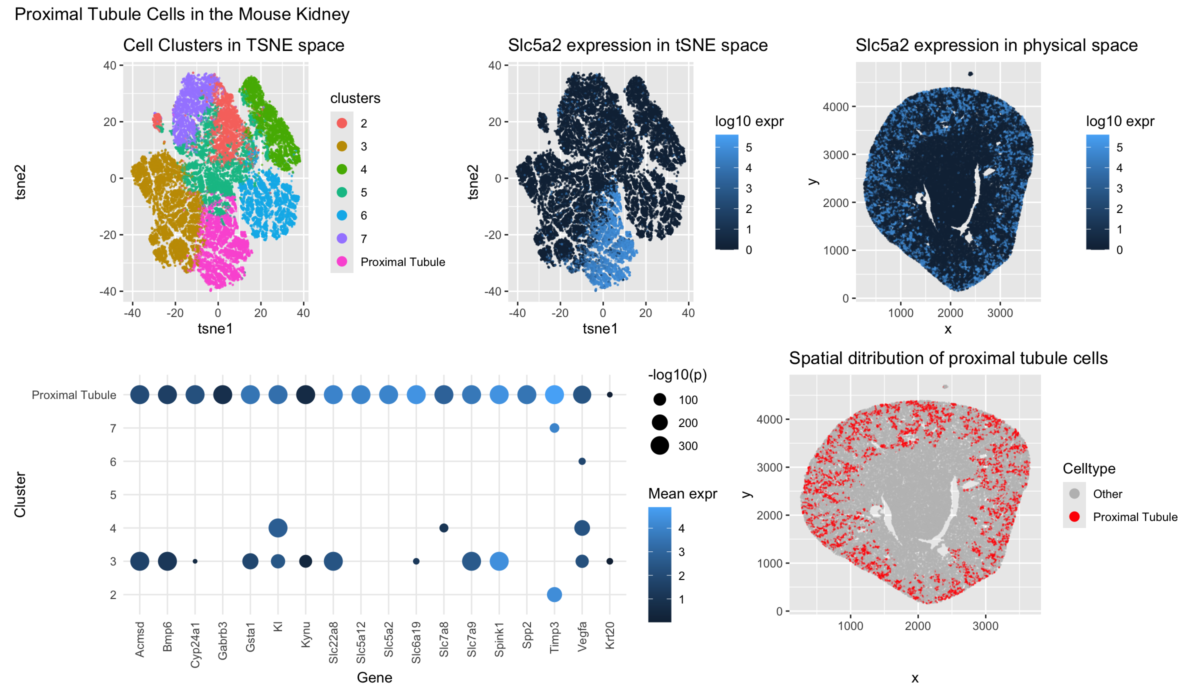
I created a data visualization with the goal of identifying the cluster of cells representing the proximal tubule in mouse kidneys using the Xenium dataset. (top left) I projected the cells into tSNE space and used kmeans clustering with 7 centers to show the multiple cell types in a mouse kidney. Of which, downstream analysis showed that cluster 1 represented proximal tubule cells, thus it was relabeled to reflect this. (top middle) I then used the Wilcox test to identify one of the most uniquely upregulated genes, Slc5a2, in the proximal tubule cluster and plotted its expression in tSNE space. (top right) I then plotted Slc5a2 expression in physical space. (bottom left) Using the Wilcox test, I identified a gene set that was both highly upregulated with statistical significance in the proximal tubule cluster. I plotted both its expression represented by bubble saturation and significance by bubble size. (bottom right) I then plotted the cluster of cells I determiend to be proximal tubule cells in physical space.
According to this paper there are 7 clusters (excluding immune cells). https://pmc.ncbi.nlm.nih.gov/articles/PMC9233501/ Therefore, I used k-means clustering of k=7 in my dataset to differentiate these cells. Then, I isolated cluster 1 and examined its differentially upregulated genes using an assymetric Wilcox test and looking for genes that are upregulated with a p-value <0.001. Then, by filtering for genes that are significantly upregulated with statistical significance, I could create a set of genes that were most highly upregulated in cluster 1. I finally determined that cluster 1 (renamed to Proximal Tubule) contained cells that had proximal tubule cell identity.
Slc5a2 is a canonical proximal tubule marker. I localizes on the brush border membrane of the early proximal tubule in mice, mediating glucose reabsorption and is considered one of the most definitive marker for S1/S2 proximal tubule segments. In my data, it was also highly specific to my ‘Proximal Tubule’ cluster. It also localized to a physical region of the outer renal cortex that is consistent with proximal tubule development. https://pmc.ncbi.nlm.nih.gov/articles/PMC3014039/
Slc6a19 is primarily expressed in early proximal tubules where it mediates reabsorption of amino acids. It is also highly specific to my ‘Proxiumal Tubule’ cluster.https://pmc.ncbi.nlm.nih.gov/articles/PMC9484999/
Spp2 is also highly specific to my cluster in proximal tubules. Mouse Cre strains with Spp2-GFP expression also primarily localize in the proximal tubules of the kidney. https://www.jax.org/strain/025209
Many of the other genes like Cyp24a1, KI, Acmsd, and Slc22a8 have also been observed in mouse proximal tubule monoculture in vitro. https://journals.lww.com/jasn/fulltext/2021/01000/transcriptomes_of_major_proximal_tubule_cell.11.aspx
1
2
3
4
5
6
7
8
9
10
11
12
13
14
15
16
17
18
19
20
21
22
23
24
25
26
27
28
29
30
31
32
33
34
35
36
37
38
39
40
41
42
43
44
45
46
47
48
49
50
51
52
53
54
55
56
57
58
59
60
61
62
63
64
65
66
67
68
69
70
71
72
73
74
75
76
77
78
79
80
81
82
83
84
85
86
87
88
89
90
91
92
93
94
95
96
97
98
99
100
101
102
103
104
105
106
107
108
109
110
111
112
113
114
115
116
117
118
119
library(ggplot2)
library(Rtsne)
library(dplyr)
library(patchwork)
data <- read.csv('/Users/willli/Documents/BME 25-26/Genomic Data Visualization/genomic-data-visualization-2026/data/Xenium-IRI-ShamR_matrix.csv.gz')
data <- data[sample(1:nrow(data), 40000),]
pos <- data [,c('x', 'y')]
rownames(pos) <- data[, 1]

gexp <- data[, 4:ncol(data)]
totgexp <- rowSums(gexp)
mat <- log10(gexp/totgexp * 10^6 + 1)


## PCAs
pcs <- prcomp(mat, center=T, scale=F)
toppcs <- pcs$x[, 1:20]
tsne <- Rtsne::Rtsne(toppcs, dims = 2, perpexity = 30)
emb <- tsne$Y
rownames(emb) <- rownames(mat)
colnames(emb) <- c('tsne1', 'tsne2')


clusters <- as.factor(kmeans(toppcs, centers=7)$cluster)
df <- data.frame(emb, clusters, pos, pcs$x, gene=mat[ , 'Spp2'])

ggplot(df, aes(x = tsne1, y = tsne2, col = clusters)) + geom_point( size = 0.1, alpha = 0.5)
ggplot(df, aes(x = x, y = y, col = clusters)) + geom_point( size = 0.1, alpha = 0.5)

vg <- apply(mat, 2, var)
vargenes <- names(sort(vg, decreasing=TRUE))
head(vargenes)
ggplot(df, aes(x=tsne1, y=tsne2, col=gene)) + geom_point(size=0.5, alpha=0.5)
ggplot(df, aes(x=tsne1, y=tsne2, col=clusters)) + geom_point(size=0.5, alpha=0.5)

clusterofinterest <- names(clusters)[clusters == 1]
othercells <- names(clusters)[clusters != 1]

out <- sapply(colnames(mat), function(gene) {
  x1 <- mat[clusterofinterest, gene]
  x2 <- mat[othercells, gene]
  wilcox.test(x1, x2, alternative='greater')$p.value
})
degs <- out[out < 1e-3]
degs <- sort(degs)

proximal_tubule_genes <- c( "Spp2", "Slc7a8", "Slc6a19", "Slc5a2", "Slc5a12")
p <- list()
for(gene in proximal_tubule_genes){
  print(gene)
  df <- data.frame(emb, pos, clusters, gene=mat[,gene])
  p[[gene]] <- ggplot(df, aes(x=tsne1, y=tsne2, col=gene)) + geom_point(size=0.5, alpha=0.5) + labs(title = gene)
  print(p[[gene]])
}

df <- df %>%
  mutate(clusters = ifelse(clusters == 1, "Proximal Tubule", as.character(clusters)))

slc5a2 <- ggplot(df, aes(x=tsne1, y=tsne2, col=mat[, 'Slc5a2'])) + geom_point(size=0.2, alpha=0.5) +
  labs(title = 'Slc5a2 expression in tSNE space', color = 'log10 expr')
slc5a2_xy <- ggplot(df, aes(x=x, y=y, col=mat[, 'Slc5a2'])) + geom_point(size=0.2, alpha=0.5) +
  labs(title = 'Slc5a2 expression in physical space', color = 'log10 expr')
cluster_plot <- ggplot(df, aes(x=tsne1, y=tsne2, col=clusters)) + geom_point(size=0.2, alpha=0.5) +
  labs(title = 'Cell Clusters in TSNE space') + guides(color = guide_legend(override.aes = list(size = 3, alpha = 1)))
section_view <- ggplot(df, aes(x=x, y=y,
                               col = ifelse(clusters == "Proximal Tubule", "Proximal Tubule", "Other"))) +
                              scale_color_manual(values = c("Proximal Tubule" = "red", "Other" = "grey")) +
                              geom_point(size=0.1, alpha=0.5) +
                              labs(title = 'Spatial ditribution of proximal tubule cells', color = 'Celltype') +
                              guides(color = guide_legend(override.aes = list(size = 3, alpha = 1)))

selected_genes <- names(degs)

avg <- sapply(selected_genes, function(g) tapply(mat[, g], clusters, mean, na.rm = TRUE))
avg_long <- as.data.frame(as.table(avg))
colnames(avg_long) <- c("cluster", "gene", "avg_expr")


sig_out <- data.frame(matrix(nrow = length(degs)))

for (cl in sort(unique(clusters))) {
  idx1 <- which(clusters == cl)
  idx2 <- which(clusters != cl)

  sig_out[cl] <- sapply(selected_genes, function(gene) {
    x1 <- mat[idx1, gene]
    x2 <- mat[idx2, gene]
    res <- wilcox.test(x1, x2, alternative='greater')$p.value
    -log10(res)
  })
}
rownames(sig_out) <- selected_genes

df_dot <- avg_long
df_dot$sig <- sapply(1:nrow(avg_long), function(i) {
  sig_out[avg_long$gene[i], as.character(avg_long$cluster[i])]
})
df_dot$sig[is.infinite(df_dot$sig)] <- max(df_dot$sig[is.finite(df_dot$sig)])

df_dot <- df_dot %>%
  group_by(gene) %>%
  filter(cluster[which.max(avg_expr)] == 1) %>%
  ungroup()

df_dot <- df_dot %>%
  mutate(cluster = ifelse(cluster == 1, "Proximal Tubule", as.character(cluster)))

dot_plot <- ggplot(df_dot, aes(x = gene, y = cluster)) +
  geom_point(aes(size = ifelse(sig >= 3, sig, NA), color = avg_expr )) +
  theme_minimal() +
  theme(axis.text.x = element_text(angle = 90, vjust = 0.5, hjust = 1)) +
  labs(x = "Gene", y = "Cluster", color = "Mean expr", size = "-log10(p)" )


(cluster_plot + slc5a2 + slc5a2_xy) /
  (dot_plot + section_view + plot_layout(widths = c(2, 1))) +
  plot_annotation(title = "Proximal Tubule Cells in the Mouse Kidney")