Identification of Thick Ascending Limb Cells in Visium Spatial Transcriptomics of Mouse Kidney

1. Describe your figure briefly so we know what you are depicting (you no longer need to use precise data visualization terms as you have been doing). Write a description to convince me that your cluster interpretation is correct. Your description may reference papers and content that allowed you to interpret your cell cluster as a particular cell-type. You must provide attribution to external resources referenced. Links are fine; formatted references are not required. You must include the entire code you used to generate the figure so that it can be reproduced.
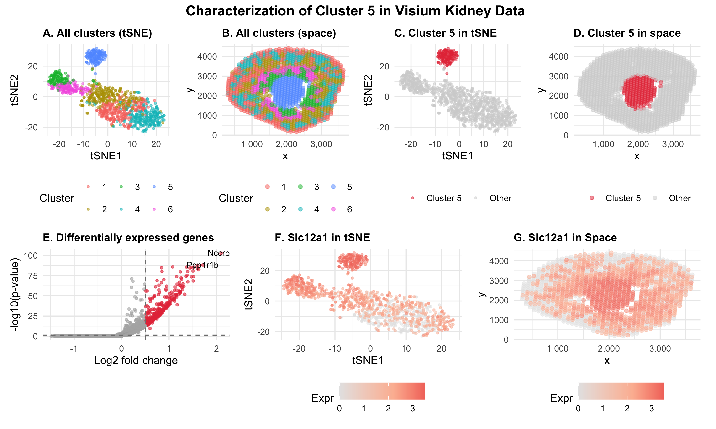
My multi-panel figure identifies Cluster 5 by using k-means clustering (k=6) of the Visium kidney dataset. The gene expression data was normalized using CPM and log10-transformed. Then, the top 500 most variable genes were selected for dimensionality reduction. Next, PCA was performed on the selected genes followed by tSNE on the first 15 PCs. I tested k = 5, 6, and 7 for k-means clustering and chose k=6 because it produced well-separated clusters without over-splitting. At k=7, two clusters appeared adjacent in tSNE space and likely represented the same transcriptional group.
In the figure, I am visualizing both quantitative and categorical data across the seven panels. The quantitative data includes tSNE embeddings, spatial x coordinates, spatial y coordinates, gene expression levels, log2 fold change, and -log10 p-values. The categorical data is cluster identity. The geometric primitive of points is used throughout all panels, where each point represents a Visium spot (panels A-D, F-G) or a gene (panel E).
Panels A and B make salient the overall transcriptional and spatial organization of the tissue by showing all six clusters in tSNE and physical space. The x and y position encode either tSNE coordinates or spatial coordinates, and the visual channel of color hue encodes each categorical cluster. The Gestalt principle of similarity is used to allow viewers to quickly identify the same cluster by shared hue. Panel B focuses on making it salient that the clusters are not randomly distributed across the tissue but correspond to spatially coherent regions. As a result, the Gestalt principle of proximity reveals that transcriptionally similar spots also tend to co-localize, reflecting anatomical structures.
Panels C and D make salient both the transcriptional identity and spatial localization of Cluster 5 compared to the other cells. This is done with color hue encoding of red for Cluster 5 and grey for all others. A compact, well-separated group in the tSNE space can be seen, showing Cluster 5. This means cluster 5 is transcriptionally distinct from all the other cells. In addition, the cluster tightly localizes in physical space to the center medulla of the kidney.
Panel E makes salient which genes are upregulated in Cluster 5. It is a volcano plot showing differentially expressed genes that were identified with a one-sided Wilcoxon rank-sum test. Each point represents a gene with the visual channel of color hue identifying differentially expressed genes as red compared to others as grey. The x-axis position encodes log2-fold change while the y-axis position encodes -log10 p-value. This shows there are many genes are significantly upregulated in Cluster 5, with the top genes being Nccrp1 and Ppp1r1b.
Panels F and G makes salient the spatial expression pattern of Slc12a1, a typical marker of the thick ascending limb of the kidney that was one of the most upregulated genes in Cluster 5. The visual channel of color saturation from light to dark red is used to encode the quantitative gene expression level. Although Slc12a1 expression is found in many other cells, it can be seen that it is concentrated in Cluster 5 for both the tSNE and physical space, using the Gestalt principle of proximity for high-expression spots.
I interpreted that Cluster 5 likely represents cells for the thick ascending limb (TAL) of the loop of Henle. Slc12a1 encodes the Na-K-2Cl cotransporter (NKCC2) which is commonly used as the defining marker of the TAL. It is also the molecular target of loop diuretics like furosemide found in the TAL (https://www.genecards.org/cgi-bin/carddisp.pl?gene=SLC12A1). In addition, another highly expressed gene, not labeled in the visualization, Umod encodes uromodulin (Tamm-Horsfall protein). This is the most abundant protein found in normal urine and is produced only by TAL cells. As a result, it is a TAL marker (https://www.proteinatlas.org/ENSG00000169344-UMOD). Ppp1r1b (DARPP-32) is found in the renal outer medulla and specifically expressed in the TAL. It regulates Na+-K+-ATPase activity after dopamine stimulation (Blau et al., 1995; https://scholars.mssm.edu/en/publications/darpp-32-promoter-directs-transgene-expression-to-renal-thick-asc-2). Nccrp1 (FBXO50) is an F-box associated domain containing protein that is highly expression in kidney when tested on mouse tissues (Kallio et al., 2011; https://omim.org/entry/615901).
The spatial localization of Cluster 5 to the central medulla is consistent with the TAL. The TAL goes across the outer and inner medulla. The high expression of Slc12a1 and Umod along with Ppp1r1b and the medulla spatial localization, provides strong evidence that Cluster 5 corresponds to TAL cells.
2. Code
1
2
3
4
5
6
7
8
9
10
11
12
13
14
15
16
17
18
19
20
21
22
23
24
25
26
27
28
29
30
31
32
33
34
35
36
37
38
39
40
41
42
43
44
45
46
47
48
49
50
51
52
53
54
55
56
57
58
59
60
61
62
63
64
65
66
67
68
69
70
71
72
73
74
75
76
77
78
79
80
81
82
83
84
85
86
87
88
89
90
91
92
93
94
95
96
97
98
99
100
101
102
103
104
105
106
107
108
109
110
111
112
113
114
115
116
117
118
119
120
121
122
123
124
125
126
127
128
129
130
131
132
133
134
135
136
137
138
139
140
141
142
143
144
145
146
147
148
149
150
151
152
153
154
155
156
157
158
159
160
161
162
163
164
165
166
167
168
169
170
171
172
173
174
175
176
177
178
179
180
181
182
183
184
185
186
187
188
189
190
191
192
193
194
195
196
197
# LOAD DATA
setwd("/Users/emmameihofer/Documents/GitHub/genomic-data-visualization-2026")
data <- read.csv("data/Visium-IRI-ShamR_matrix.csv.gz")
pos <- data[, c('x', 'y')]
rownames(pos) <- data[, 1]
gexp <- data[, 4:ncol(data)]
rownames(gexp) <- data[, 1]

# NORMALIZE
totgexp <- rowSums(gexp)
mat <- log10(gexp / totgexp * 1e6 + 1)  # CPM + log10

# VARIABLE GENE SELECTION
vg <- apply(mat, 2, var)
vargenes <- names(sort(vg, decreasing = TRUE)[1:500])
matsub <- mat[, vargenes]

# PCA
pcs <- prcomp(matsub, center = TRUE, scale. = FALSE)

# tSNE
set.seed(42)  # reproducibility
tsne <- Rtsne::Rtsne(pcs$x[, 1:15], dims = 2, perplexity = 30)
emb <- tsne$Y
rownames(emb) <- rownames(matsub)
colnames(emb) <- c('tSNE1', 'tSNE2')

# K-MEANS CLUSTERING
set.seed(42)
k <- 6
km <- kmeans(pcs$x[, 1:15], centers = k)
clusters <- as.factor(km$cluster)

# Pick CLUSTER OF INTEREST
library(ggplot2)

# Quick look at clusters in tSNE and space
df_explore <- data.frame(pos, emb, cluster = clusters)
print(ggplot(df_explore, aes(x = tSNE1, y = tSNE2, col = cluster)) +
        geom_point(size = 1.5) + theme_minimal() + ggtitle("Clusters in tSNE"))
print(ggplot(df_explore, aes(x = x, y = y, col = cluster)) +
        geom_point(size = 2) + coord_fixed() + theme_minimal() + ggtitle("Clusters in space"))

cluster_of_interest <- 5  # <--- CHANGE THIS after exploring

# DIFFERENTIAL EXPRESSION (Wilcoxon test)
cells_in <- names(clusters)[clusters == cluster_of_interest]
cells_out <- names(clusters)[clusters != cluster_of_interest]

# Test all genes for upregulation in cluster of interest
de_pvals <- sapply(colnames(mat), function(gene) {
  wilcox.test(mat[cells_in, gene],
              mat[cells_out, gene],
              alternative = 'greater')$p.value
})

# Compute log2 fold change
mean_in <- colMeans(mat[cells_in, ])
mean_out <- colMeans(mat[cells_out, ])
log2fc <- mean_in - mean_out  # already log-scale, so difference ~ log fold change

de_results <- data.frame(
  gene = names(de_pvals),
  pval = de_pvals,
  log2fc = log2fc,
  neglog10p = -log10(de_pvals)
)
de_results <- de_results[order(de_results$pval), ]

cat("Top 15 upregulated genes in cluster", cluster_of_interest, ":\n")
print(head(de_results, 15))

# Pick the top gene for visualization
top_gene <- "Slc12a1"
cat("\nTop marker gene:", top_gene, "\n")

# MULTI-PANEL FIGURE
library(ggplot2)
library(patchwork)

# Define a color for the cluster of interest
cluster_binary <- ifelse(clusters == cluster_of_interest,
                         paste0("Cluster ", cluster_of_interest),
                         "Other")
cluster_binary <- factor(cluster_binary,
                         levels = c(paste0("Cluster ", cluster_of_interest), "Other"))

# Build the data frame
df <- data.frame(
  pos,
  emb,
  PC1 = pcs$x[, 1],
  PC2 = pcs$x[, 2],
  cluster = clusters,
  cluster_highlight = cluster_binary,
  top_gene_expr = mat[, top_gene]
)

# Color palette
highlight_cols <- c("#E63946", "#D3D3D3")
names(highlight_cols) <- levels(cluster_binary)

# Shared theme for consistency
theme_hw <- theme_minimal(base_size = 11) +
  theme(plot.title = element_text(face = "bold", size = 11),
        legend.position = "bottom",
        plot.margin = margin(5, 10, 5, 5))

# Panel A: All clusters in tSNE
pA <- ggplot(df, aes(x = tSNE1, y = tSNE2, col = cluster)) +
  geom_point(size = 0.8, alpha = 0.5) +
  labs(title = "A. All clusters (tSNE)", color = "Cluster") +
  theme_hw

# Panel B: All clusters in physical space
pB <- ggplot(df, aes(x = x, y = y, col = cluster)) +
  geom_point(size = 1.5, alpha = 0.5) +
  scale_x_continuous(labels = scales::comma) +
  labs(title = "B. All clusters (space)", color = "Cluster") +
  theme_hw

# Panel C: Cluster highlighted in tSNE
pC <- ggplot(df, aes(x = tSNE1, y = tSNE2, col = cluster_highlight)) +
  geom_point(size = 0.8, alpha = 0.5) +
  scale_color_manual(values = highlight_cols) +
  labs(title = "C. Cluster 5 in tSNE", color = NULL) +
  theme_hw

# Panel D: Cluster highlighted in physical space
pD <- ggplot(df, aes(x = x, y = y, col = cluster_highlight)) +
  geom_point(size = 1.5, alpha = 0.5) +
  scale_color_manual(values = highlight_cols) +
  scale_x_continuous(labels = scales::comma) +
  labs(title = "D. Cluster 5 in space", color = NULL) +
  theme_hw

# Panel E: Volcano plot of DE genes
de_results$significant <- de_results$pval < 0.05 & de_results$log2fc > 0.5
top5 <- head(de_results$gene, 5)
de_results$label <- ifelse(de_results$gene %in% top5, de_results$gene, "")

pE <- ggplot(de_results, aes(x = log2fc, y = neglog10p)) +
  geom_point(aes(col = significant), size = 1, alpha = 0.6) +
  scale_color_manual(values = c("TRUE" = "#E63946", "FALSE" = "grey70")) +
  geom_text(aes(label = label), size = 3, nudge_y = 0.5, check_overlap = TRUE) +
  geom_hline(yintercept = -log10(0.05), linetype = "dashed", color = "grey50") +
  geom_vline(xintercept = 0.5, linetype = "dashed", color = "grey50") +
  labs(title = "E. Differentially expressed genes",
       x = "Log2 fold change", y = "-log10(p-value)") +
  theme_hw +
  theme(legend.position = "none")

# Sort so high-expression spots are drawn last (on top)
df_sorted <- df[order(df$top_gene_expr), ]

# Panel F: Top gene in tSNE
pF <- ggplot(df_sorted, aes(x = tSNE1, y = tSNE2, col = top_gene_expr)) +
  geom_point(size = 0.8, alpha = 0.5) +
  scale_color_gradient2(low = "grey90", mid = "#FCBBA1", high = "#E63946",
                        midpoint = median(df$top_gene_expr)) +
  labs(title = paste0("F. ", top_gene, " in tSNE"), color = "Expr") +
  theme_hw

# Panel G: Top gene in physical space
pG <- ggplot(df_sorted, aes(x = x, y = y, col = top_gene_expr)) +
  geom_point(size = 1.5, alpha = 0.5) +
  scale_color_gradient2(low = "grey90", mid = "#FCBBA1", high = "#E63946",
                        midpoint = median(df$top_gene_expr)) +
  scale_x_continuous(labels = scales::comma) +
  labs(title = paste0("G. ", top_gene, " in Space"), color = "Expr") +
  theme_hw

# ASSEMBLE PLOT AND SAVE
# Layout:
# Row 1 (4 panels): A (all tSNE) | B (all space) | C (cluster tSNE) | D (cluster space)
# Row 2 (3 panels): E (volcano)  | F (gene tSNE) | G (gene space)

top_row <- pA + pB + pC + pD + plot_layout(nrow = 1)
bot_row <- pE + pF + pG + plot_layout(nrow = 1)

final_fig <- (top_row / bot_row) +
  plot_annotation(
    title = paste0('Characterization of Cluster ', cluster_of_interest,
                   ' in Visium Kidney Data'),
    theme = theme(plot.title = element_text(face = "bold", size = 14, hjust = 0.5))
  )

ggsave('hw3_figure.png', final_fig, width = 22, height = 11, dpi = 300, bg = "white")
cat("\nFigure saved to hw3_figure.png\n")

# SUMMARY — Top marker genes
cat("\n=== TOP 20 MARKER GENES ===\n")
print(head(de_results[, c('gene', 'pval', 'log2fc')], 20))
cat("\nSearch these gene names + 'kidney' in literature to identify the cell type.\n")
cat("Useful resources: The Human Protein Atlas, GeneCards, PubMed\n")

ggsave("/Users/EmmaMeihofer/Downloads/emeihof1_HW3.png", width = 10, height = 6)