Identification and Spatial Characterization of a Transcriptionally Distinct Cell Cluster

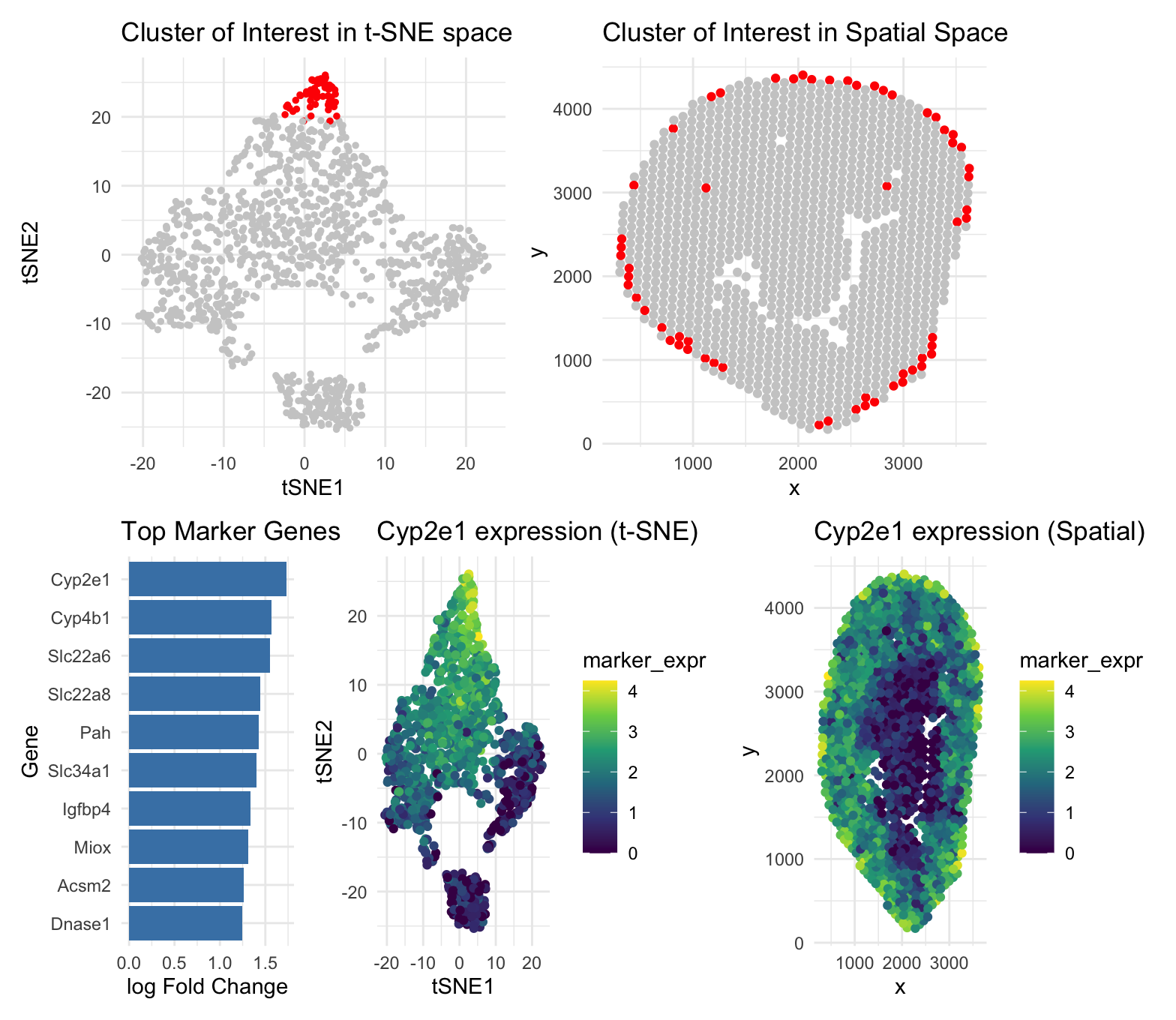
This figure explores a transcriptionally distinct cluster of Visium spots identified using PCA, t-SNE, and k-means clustering. In the t-SNE plot (top left), the cluster of interest appears as a compact and well-separated group, indicating a shared gene expression profile. The corresponding spatial plot (top right) shows that these spots are concentrated near the tissue periphery, demonstrating that the transcriptional clustering aligns with a coherent anatomical region. The bar plot of differentially expressed genes (bottom left) highlights marker genes such as Cyp2e1, Cyp4b1, Slc22a6, Slc22a8, and Pah, which are associated with metabolic and detoxification functions. Expression of Cyp2e1 is shown in both reduced dimensional space and physical space (bottom middle and bottom right), where high expression is largely restricted to the selected cluster and spatially enriched in the same peripheral tissue regions. Together, these panels show strong agreement between transcriptional patterns and spatial organization, supporting the interpretation that this cluster represents a metabolically specialized cell population or functional tissue zone.
5. Code (paste your code in between the ``` symbols)
1
2
3
4
5
6
7
8
9
10
11
12
13
14
15
16
17
18
19
20
21
22
23
24
25
26
27
28
29
30
31
32
33
34
35
36
37
38
39
40
41
42
43
44
45
46
47
48
49
50
51
52
53
54
55
56
57
58
59
60
61
62
63
64
65
66
67
68
69
70
71
72
73
74
75
76
77
78
79
80
81
82
83
84
85
86
87
88
89
90
91
92
93
94
95
96
97
98
99
100
101
102
library(tidyverse)
library(Rtsne)
library(patchwork)
data <- read.csv("~/Desktop/Visium-IRI-ShamR_matrix.csv.gz")
meta <- numeric_data [, 1:2]
expr <- numeric_data [, -c(1,2)]
expr <- as.matrix(expr)
mode(expr) <- 'numeric'

# Library size normalization (CP10K) + log1p
lib_size <- rowSums(expr)
expr_norm <- log1p(t(t(expr) / lib_size * 1e4))

gene_vars <- apply(expr_norm, 2, var)
top_genes <- names(sort(gene_vars, decreasing = TRUE))[1:2000]

expr_hvg <- expr_norm[, top_genes]
pca <- prcomp(expr_hvg, scale. = TRUE)
pca_df <- as.data.frame(pca$x[, 1:20])
set.seed(1)
tsne <- Rtsne(
  pca_df,
  dims = 2,
  perplexity = 30,
  verbose = TRUE,
  max_iter = 500
)

tsne_df <- data.frame(
  tSNE1 = tsne$Y[,1],
  tSNE2 = tsne$Y[,2]
)

#k-means clustering
set.seed(1)
k <- 6
clusters <- kmeans(pca_df[,1:10], centers = k)$cluster

tsne_df$cluster <- factor(clusters)
meta$cluster <- factor(clusters)
cluster_of_interest <- "3"


cluster_cells <- clusters == cluster_of_interest

logFC <- colMeans(expr_norm[cluster_cells, ]) -
  colMeans(expr_norm[!cluster_cells, ])

de_genes <- sort(logFC, decreasing = TRUE)
top_markers <- names(de_genes)[1:10]
top_markers
marker_gene <- top_markers[1]


p1 <- ggplot(tsne_df, aes(tSNE1, tSNE2, color = cluster == cluster_of_interest)) +
  geom_point(size = 1) +
  scale_color_manual(values = c("grey80", "red")) +
  labs(title = "Cluster of Interest in t-SNE space") +
  theme_minimal() +
  theme(legend.position = "none")


p2 <- ggplot(meta, aes(x, y, color = cluster == cluster_of_interest)) +
  geom_point(size = 1.5) +
  scale_color_manual(values = c("grey80", "red")) +
  labs(title = "Cluster of Interest in Spatial Space") +
  theme_minimal() +
  theme(legend.position = "none")

de_df <- data.frame(
  gene = top_markers,
  logFC = de_genes[top_markers]
)

p3 <- ggplot(de_df, aes(reorder(gene, logFC), logFC)) +
  geom_col(fill = "steelblue") +
  coord_flip() +
  labs(title = "Top Marker Genes", x = "Gene", y = "log Fold Change") +
  theme_minimal()

tsne_df$marker_expr <- expr_norm[, marker_gene]

p4 <- ggplot(tsne_df, aes(tSNE1, tSNE2, color = marker_expr)) +
  geom_point(size = 1.5) +
  scale_color_viridis_c() +
  labs(title = paste(marker_gene, "expression (t-SNE)")) +
  theme_minimal()

meta$marker_expr <- expr_norm[, marker_gene]

p5 <- ggplot(meta, aes(x, y, color = marker_expr)) +
  geom_point(size = 1.5) +
  scale_color_viridis_c() +
  labs(title = paste(marker_gene, "expression (Spatial)")) +
  theme_minimal()

final_plot <- (p1 | p2) /
  (p3 | p4 | p5)

final_plot
(Please do not copy. I did not do a good job on this HW.)