Highlighting Proximal Convoluted Tubule Segments with SLC gene family

Description
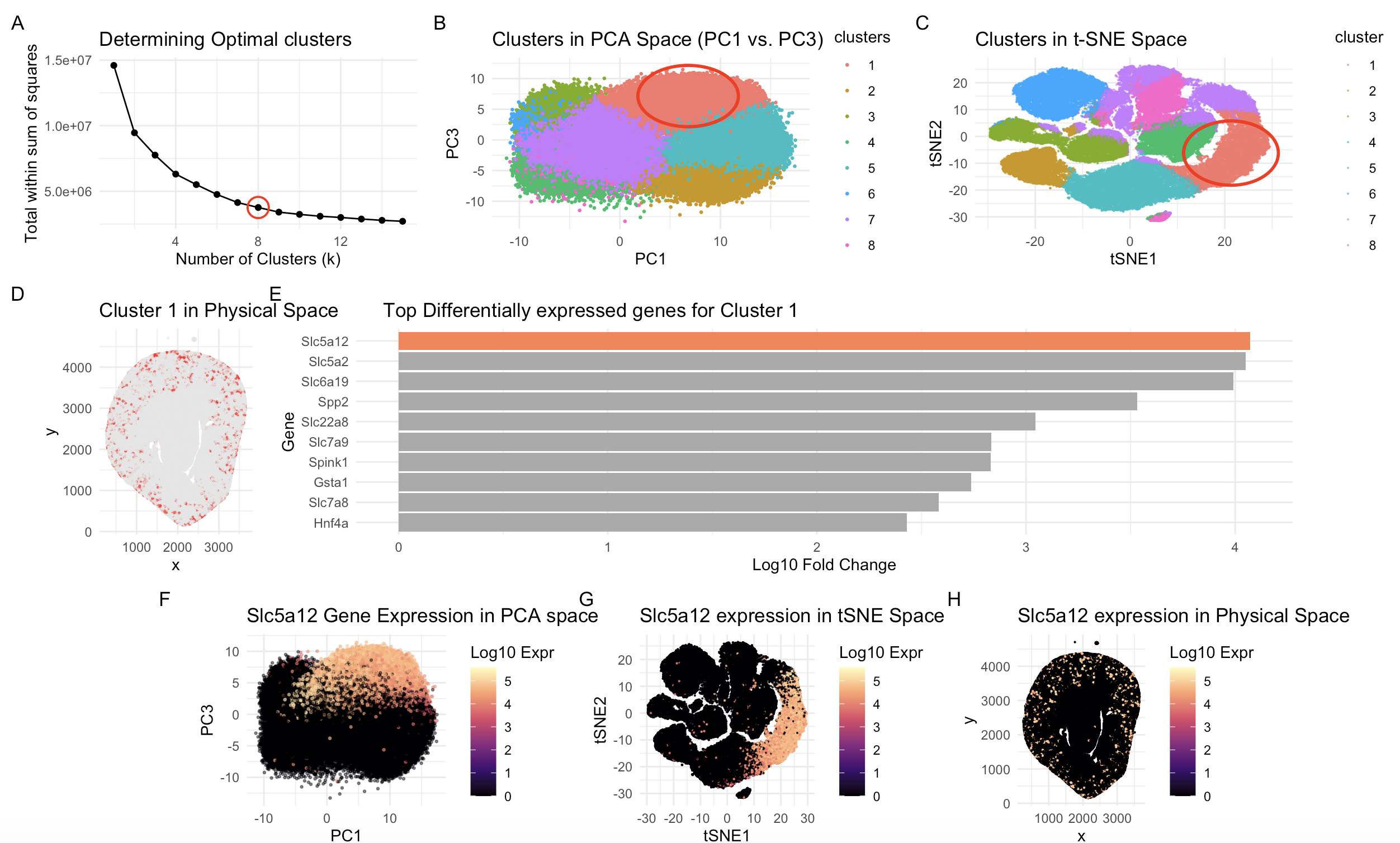
This multi-panel visualization combines a multitude of concepts essential in spatial transcriptomic data analysis and visualization, including normalization/log-transformation, dimensionality reduction, k-means clustering, and differential expression. By combining these methods, we were able to identify and support the biological identity of a specific cell population within a kidney coronal section.
A transcriptionally distinct cluster of cells, Cluster 1, was chosen as I was curious of its presence between two islands in the tSNE space. It is consistently depicted in a coral-red tone to allow viewers to easily follow along in both PCA and tSNE space (Panel B, C, D). Additionally, the Gestalt principle of enclosure with a red circle makes clear which cluster is relevant amongst many others.
Based on the high differential expression of genes in the Slc family, with the 3 genes with the highest log fold change being Slc5a12, Slc5a2, Slc6a19, there is high reason to suspect the Solute Carrier Gene’s function holds high relevance in this cell type (Panel E). There are 3 additional Slc genes in ranks 5, 6, and 9 as well. From literature, the solute carrier (SLC) family of proteins is responsible for much of the transport of ions and organic molecules along the renal tubule, with the highest concentration and diversity located in the proximal tubule.
This is supported in Panel D with Cluster 1 expression located across the renal cortex in a tubular pattern. A classification system developed for the proximal tubules divides them into proximal convoluted and straight segments (PCTs and PSTs, respectively). To speculate further for cell type, I believe Cluster 1 signifies PCT cells of proximal tubules, rather than PST. According to literature, “The PCT segment has important transporters specific to this segment, such as Slc5a2 and Slc5a12”. These happen to be the top 2 most differentially expressed genes in our data for this cluster. Additionally, “SLC6A19 is found in the early portion of the proximal tubule”, which further aligns with our speculation that we are in PCT not PST. SLC6A19 is the third most upregulated gene.
Slc5a12 was chosen as a representative gene to explore within the PCA, tSNE, and physical space in panels F, G, H respectively. With a Magma scale, more information regarding the log-transformed expression levels is encoded. There is high alignment between cluster 1 location and gene across the 3 graphs. However, gene expression does expand slightly beyond cluster boundaries, I speculate this is as according to literature “There is no ‘sharp’ anatomical boundary, as the segments transform gradually”, so there might be some overlap with a cluster representing the straight segments.
On another note, Panel A shows an elbow plot for determining an optimal k by calculating the total within-cluster sum of squares from k=1 to 15. Since it is speculative where the sharp drop stops and flattening begins, I ran the code with k=6,7,8, and 9 and settled on 8. While I recognize there are some areas that are not completely distinct clusters, k=8 seemed to best trade-off between zones and avoiding over-clustering. PCA plot in panel B depicts PC1 vs PC3 chosen over PC1 vs PC2 because PC3 captured more specific variance that was able to separate the clusters.
References
-Lewis, S., Chen, L., Raghuram, V., Khundmiri, S. J., Chou, C. L., Yang, C. R., & Knepper, M. A. (2021). “SLC-omics” of the kidney: solute transporters along the nephron. American journal of physiology. Cell physiology, 321(3), C507–C518. https://doi.org/10.1152/ajpcell.00197.2021
-https://www.proteinatlas.org/ENSG00000148942-SLC5A12
-https://medlineplus.gov/genetics/gene/slc5a1/
-https://maayanlab.cloud/Harmonizome/gene/SLC5A12
Code (paste your code in between the ``` symbols)
1
2
3
4
5
6
7
8
9
10
11
12
13
14
15
16
17
18
19
20
21
22
23
24
25
26
27
28
29
30
31
32
33
34
35
36
37
38
39
40
41
42
43
44
45
46
47
48
49
50
51
52
53
54
55
56
57
58
59
60
61
62
63
64
65
66
67
68
69
70
71
72
73
74
75
76
77
78
79
80
81
82
83
84
85
86
87
88
89
90
91
92
93
94
95
96
97
98
99
100
101
102
103
104
105
106
107
108
109
110
111
112
113
114
115
116
117
118
119
120
121
122
123
124
125
126
127
128
129
130
131
132
133
134
135
136
137
138
139
library(ggplot2)
library(patchwork)
library(Rtsne)

data <- read.csv('~/Desktop/GDV/Xenium-IRI-ShamR_matrix.csv.gz')
pos <- data[,c('x','y')]
rownames(pos) <- data[,1]
gexp <- data[,4:ncol(data)]
rownames(gexp) <- data[,1]

totgexp <- rowSums(gexp)
#normalizing the data
mat <- log10(gexp/totgexp * 1e6 + 1)

#PCA
pcs <- prcomp(mat, center = TRUE, scale = FALSE)
plot(pcs$sdev[1:50]) #first 10 pcs chosen based on this plot

#tSNE
set.seed(42)
tsne <- Rtsne::Rtsne(pcs$x[, 1:10], dims=2, perplexity=30, verbose=TRUE) #verbose parameter added for troubleshooting
emb <- tsne$Y
rownames(emb) <- rownames(mat)
colnames(emb) <- c('tSNE1', 'tSNE2')
head(emb)

# Determining optimal k
#Prompt to Gemini "create a for loop that calculates the tot.withiness for k clusters"
wss <- sapply(1:15, function(k){kmeans(pcs$x[,1:10], centers=k, nstart=10)$tot.withinss})
elbow_df <- data.frame(k=1:15, wss=wss)
p_elbow <- ggplot(elbow_df, aes(x=k, y=wss)) +
  geom_line() +
  geom_point() +
  theme_minimal() +
  labs(title="Determining Optimal clusters", x="Number of Clusters (k)", y="Total within sum of squares") +
  #Prompt to Gemini "how do I add a circle around my optimal k; how do I increase the thickness"
  geom_point(data = elbow_df[elbow_df$k == 8, ], #estimated 8 as optimal k
             aes(x=k, y=wss),
             color="red", size=6, shape=1, stroke=1)
p_elbow
clusters <- as.factor(kmeans(pcs$x[,1:10], centers = 8)$cluster)
df_clusters <- data.frame(pos, pcs$x[,1:10], emb, cluster = clusters)
p1 <- ggplot(df_clusters, aes(x=PC1, y=PC3, col=clusters)) +
  geom_point(size = 0.5) +
  theme_minimal() +
  annotate("path",
           x=mean(df_clusters$PC1[df_clusters$cluster==1]) + 5*cos(seq(0,2*pi,length.out=100)),
           y=mean(df_clusters$PC3[df_clusters$cluster==1]) + 5*sin(seq(0,2*pi,length.out=100)),
           color="red", size=1) +
  labs(title="Clusters in PCA Space (PC1 vs. PC3)")
p1
p2 <- ggplot(df_clusters, aes(x=tSNE1, y=tSNE2, col=cluster)) +
  geom_point(size = 0.1, alpha = 0.5) +
  theme_minimal() +
  labs(title="Clusters in t-SNE Space") +
  annotate("path",
           x=mean(df_clusters$tSNE1[df_clusters$cluster==1]) + 10*cos(seq(0,2*pi,length.out=100)),
           y=mean(df_clusters$tSNE2[df_clusters$cluster==1]) + 12*sin(seq(0,2*pi,length.out=100)),
           color="red", size=1)
p2
#finalize target cluster
target_cluster <- 1
#target cluster in physical space
p3 <- ggplot(df_clusters, aes(x=x, y=y, color=cluster == target_cluster)) +
  geom_point(size=0.3, alpha = 0.5) +
  coord_fixed() +
  scale_color_manual(values=c("grey90", "red")) +
  theme_minimal() +
  theme(legend.position = "none") +
  labs(title="Cluster 1 in Physical Space")
p3

#Gemini prompt: help me plot the top 10 differentially expressed genes from cluster 1. Use log fold change.
#Differential Expression for Cluster 1
cluster_dx <- which(clusters == 1)
other_dx <- which(clusters != 1)
#mean expression
mean_in <- colMeans(mat[cluster_dx, ])
mean_out <- colMeans(mat[other_dx, ])
logFC <- mean_in - mean_out #log fold change
#top 10 genes upregulated in Cluster 3
top_genes <- sort(logFC, decreasing = TRUE)[1:10]
print(top_genes)
dx_df <- data.frame(gene = names(top_genes), logFC = as.numeric(top_genes))

#AI prompt: how do I make only the Slc5a12 bar colored olive green, others gray
dx_df$color_group <- ifelse(dx_df$gene == "Slc5a12", "highlight", "other")
p4 <- ggplot(dx_df, aes(x = reorder(gene, logFC), y = logFC, fill = color_group)) +
  geom_bar(stat = "identity") +
  scale_fill_manual(values = c("highlight" = "coral", "other" = "darkgray")) +
  coord_flip() +
  theme_minimal() +
  theme(legend.position = "none") +
  labs(title = "     Top Differentially expressed genes for Cluster 1", x = "Gene", y = "Log10 Fold Change")
p4

# Gene of interest in PCA space
df_gene <- data.frame(pcs$x, gene = mat[, 'Slc5a12'])
p5 <- ggplot(df_gene, aes(x = PC1, y = PC3, color = gene)) +
  geom_point(size = 0.5, alpha = 0.5) +
  coord_fixed() +
  theme_minimal() +
  scale_color_viridis_c(option = "magma", name = "Log10 Expr") +
  labs(
    title = "Slc5a12 Gene Expression in PCA space",
    x = "PC1", y = "PC3", color = "Slc5a12 Gene Expression"
  )
p5
target_gene <- "Slc5a12"
df_clusters$gene_expr <- mat[, target_gene]

# Gene of interest in tSNE space
p6 <- ggplot(df_clusters, aes(x=tSNE1, y=tSNE2, color=gene_expr)) +
  geom_point(size=0.1, alpha=0.8) +
  coord_fixed() +
  scale_color_viridis_c(option = "magma", name = "Log10 Expr") +
  theme_minimal() +
  labs(title = "Slc5a12 expression in tSNE Space")
p6

# Gene of interest in physical space encoding gene expression levels
p7 <- ggplot(df_clusters, aes(x=x, y=y, color=gene_expr)) +
  geom_point(size=0.1) +
  coord_fixed() +
  scale_color_viridis_c(option = "magma", name = "Log10 Expr") +
  theme_minimal() +
  labs(title = paste(target_gene, "expression in Physical Space"))
p7

#reference https://patchwork.data-imaginist.com/articles/guides.html
plot <- (p_elbow | p1 | p2) /
  (p3 | p4) /
  (p5 | p6 | p7) +
  plot_layout(heights = c(1, 1.2, 1)) +
  plot_annotation(tag_levels = 'A')
plot