Identifying a kidney cortical tubule region using marker genes

The data were normalized and log-transformed. I then ran PCA on the normalized matrix, used the scree plot of PC standard deviations to pick a safe cutoff (PC = 10) for downstream analysis, and ran t-SNE. After that, I performed k-means clustering in PC space and chose k = 3 based on the elbow plot of within-cluster variance as well as my results from previous assignments.

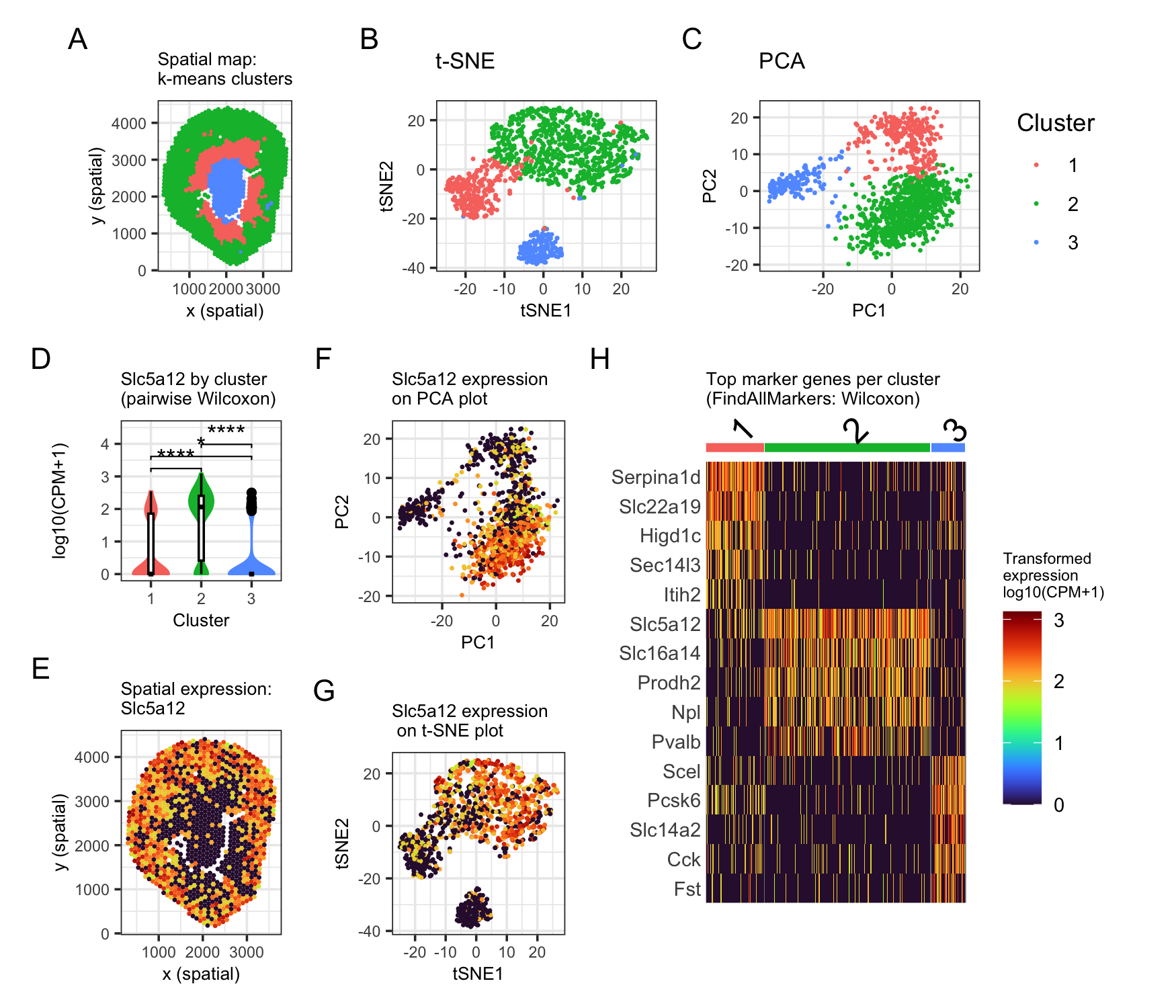
In the spatial plot, the clusters form a ring structure: cluster 2 (green) is on the outside, cluster 1 (red) is in the middle ring, and cluster 3 (blue) is in the center. This matches kidney anatomy that the outer region is cortex, while the center is medulla (A). In reduced dimensional space, the three clusters separate well, and clusters 1 and 2 are closer to each other than cluster 3 (B, C). I focus on cluster 2 as my distinct cluster of interest. Based on literature, Slc5a12 is expressed in the cortical tubule of kidney (Park et al., 2018). I therefore visualized Slc5a12 across clusters and in space (D, E, F, G). The violin plot with pairwise Wilcoxon tests shows Slc5a12 is significantly higher in cluster 2 compared with clusters 1 and 3 (D), and the spatial plots show the same pattern (E–G).

To further support this, I used Seurat FindAllMarkers (Wilcoxon) and plotted top marker genes across clusters (H). Cluster 2’s markers include Slc5a12 and other tubule-associated transport genes, supporting that this cluster is enriched for cortical tubules, most consistent with a proximal tubule region. I also note that Pvalb is a known marker of the early distal convoluted tubule, so there might be some mixing of cortical tubule segments as each Visium spot can contain multiple nearby cell types. Overall, the spatial location, outer cortex, plus the strong Slc5a12 enrichment supports the interpretation that cluster 2 corresponds to a cortex tubule region.

Jihwan Park et al. ,Single-cell transcriptomics of the mouse kidney reveals potential cellular targets of kidney disease.Science360,758-763(2018).DOI:10.1126/science.aar2131

I used AI to debug patchwork layout and formatting issues and to proofread parts of the description. Part of my data processing code is adapted from the class example code from Dr.Fan.

# hw3

library(Rtsne)
library(patchwork)
library(dplyr)
library(ggplot2)
library(gridExtra)
library(jcolors)
library(Seurat)
library(tidyverse)
library(viridis)
library(ggpubr)

setwd("/Users/tiya/Desktop/BME\ program\ info/Spring\ 2026/gemonic_data_visal")

## seperate data, normalize, PCA, tSNE, Kmeans, test the most upregulated genes in each cluster, use wilcoxon or T test to do DGE, heatmap

#### data ####
dat = read_csv("data/Visium-IRI-ShamR_matrix.csv") %>% 
  data.frame()
colnames(dat) %>% head()
dim(dat) # [1]  1224 19468
genes = setdiff(colnames(dat), c("...1", "x", "y"))
length(genes) #[1] 19465

#sort 
dat = dat %>% 
  mutate(cellnames = `...1`) %>% 
  select(-c(`...1`))
rownames(dat) = dat$cellnames

#new data
pos <- dat[,c('x', 'y')]
dim(pos) #[1] 1224    2
gexp <- dat[, genes]
dim(gexp) #[1]  1224 19465

# normalize
totgexp = rowSums(gexp)
mat <- log10(gexp/totgexp * 1e6 + 1)

# PCA
pcs <- prcomp(mat)
df <- data.frame(pcs$x, pos)
ggplot(df, aes(x=x, y=y, col=PC1)) + geom_point(cex=0.8)
plot(pcs$sdev[1:50]) #I would take a safe PC = 10
sort(abs(pcs$rotation[, 1]), decreasing = TRUE)[1:5] #Nccrp1, Ppp1r1b, Epcam, Slc12a1, Scin
sort(abs(pcs$rotation[, 2]), decreasing = TRUE)[1:5] #Serpina1f, Cyp7b1, Mep1b, Slc22a13, Irx1
pc = 10

#tSNE
set.seed(2026209)
tsne = Rtsne::Rtsne(pcs$x[, 1:pc], dims = 2, perplexity = 30)

emb = as.data.frame(tsne$Y)

#Kmeans
var = numeric(20)
for (k in 1:20) {
  km_result = kmeans(pcs$x[, 1:pc], centers = k)
  var[k] <- km_result$tot.withinss
}

plot(1:20, var, type = "b", 
     xlab = "Number of Clusters (k)", 
     ylab = "Within-cluster variance",
     main = "Elbow Method")

clusters = as.factor(kmeans(pcs$x[,1:pc], centers=3)$cluster) #picked cluster = 3 as the slope gets flat near that point
df = cbind(pos, emb, data.frame(clusters), data.frame(pcs$x)[, 1:10], mat)

ggplot(df, aes(x=PC1, y=PC2, col=clusters)) + geom_point(cex=0.8) 
ggplot(df, aes(x=x, y=y, col=clusters)) + geom_point(cex=0.8)
ggplot(df, aes(x=V1, y=V2, col=clusters)) + geom_point(cex=0.8)

#### DGE ####
ser = CreateSeuratObject(counts = t(gexp))
LayerData(ser, assay = "RNA", layer = "data") = t(mat)
ser[[]] = cbind(ser[[]], df)
Idents(ser) = ser$clusters

markers = FindAllMarkers(ser, only.pos = TRUE, min.pct = 0.25, logfc.threshold = 0.25) #by default, test.use = "wilcox"
top_markers = markers %>% 
  group_by(cluster) %>% 
  filter(avg_log2FC > 0.4 & pct.1 >= 0.25 & p_val_adj < 0.05) %>% 
  top_n(n = 5, wt = avg_log2FC)

DoHeatmap(object = ser, 
          features = top_markers$gene, slot = "data") + 
  scale_fill_viridis(option = "H")

#### put plot togethor ####
small_axes = theme(
  axis.title = element_text(size = 8),
  axis.text  = element_text(size = 7),
  plot.title = element_text(size = 10)   
)

p1 = ggplot(df, aes(x=x, y=y, col=clusters)) + 
  geom_point(cex=0.3) + 
  theme_bw() + 
  coord_fixed() + 
  labs(title = "Spatial map:\nk-means clusters",
                       x = "x (spatial)", y = "y (spatial)", color = "Cluster") + 
  small_axes + 
  theme(plot.title = element_text(size = 8)) + 
  guides(color = "none")

p2 = ggplot(df, aes(x = V1, y = V2, col=clusters)) + 
  geom_point(cex=0.3) + 
  theme_bw() + 
  labs(title = "t-SNE",
       x = "tSNE1", y = "tSNE2", color = "Cluster") + 
  small_axes + 
  guides(color = "none")

p3 = ggplot(df, aes(x = PC1, y = PC2, col=clusters)) + 
  geom_point(cex=0.3) + 
  theme_bw() + 
  labs(title = "PCA",
       x = "PC1", y = "PC2", color = "Cluster") + 
  small_axes

p4 = DoHeatmap(object = ser, 
          features = top_markers$gene, slot = "data") + 
  scale_fill_viridis(option = "H", name = "Transformed\nexpression\nlog10(CPM+1)") + 
  guides(color = "none") + 
  labs(title = "Top marker genes per cluster\n(FindAllMarkers: Wilcoxon)") + 
  theme(plot.title = element_text(size = 8), 
        legend.title =  element_text(size = 7))

p5 = ggplot(df, aes(x=x, y=y, color=Slc5a12)) + 
  geom_point(cex=0.3) + 
  theme_bw() + 
  NoLegend() + 
  scale_color_viridis(option = "H", name = "Transformed\nexpression\nlog10(CPM+1)") + 
  labs(title = "Spatial expression:\nSlc5a12",
       x = "x (spatial)", y = "y (spatial)") + 
  small_axes + 
  coord_fixed() + 
  theme(plot.title = element_text(size = 8))

p6 = ggplot(df, aes(x=clusters, y = Slc5a12, 
                    fill=clusters, color = clusters)) + 
  geom_violin() + 
  geom_boxplot(fill = "white", width = 0.1, color = "black") + 
  theme_bw() + 
  stat_compare_means(
    comparisons = combn(levels(df$clusters), 2, simplify = FALSE),
    method = "wilcox.test",
    label = "p.signif"   # or "p.format"
  ) + 
  theme(legend.position="none") + 
  labs(title = "Slc5a12 by cluster\n(pairwise Wilcoxon)",
       x = "Cluster", y = "log10(CPM+1)") + 
  small_axes + 
  ylim(0, 4.5) + 
  theme(plot.title = element_text(size = 8))

p7 = ggplot(df, aes(x = PC1, y = PC2, col=Slc5a12)) + 
  geom_point(cex=0.3) + 
  theme_bw() + 
  scale_color_viridis(option = "H") + 
  small_axes + 
  guides(color = "none") + 
  labs(title = "Slc5a12 expression\non PCA plot",
       x = "PC1", y = "PC2") + 
  theme(plot.title = element_text(size = 8))

p8 = ggplot(df, aes(x = V1, y = V2, col=Slc5a12)) + 
  geom_point(cex=0.3) + 
  theme_bw() + 
  scale_color_viridis(option = "H") + 
  small_axes + 
  guides(color = "none") + 
  labs(title = "Slc5a12 expression\n on t-SNE plot",
       x = "tSNE1", y = "tSNE2") + 
  theme(plot.title = element_text(size = 8))

#verification of wilcoxon test results 
x1 = df %>% filter(clusters == "2") %>% pull(Slc5a12)
x2 = df %>% filter(clusters == "1") %>% pull(Slc5a12)
wilcox.test(x1, x2, alternative='greater') #for 2 vs 3, W = 104426, p-value < 2.2e-16
# for 1 vs 3, W = 24664, p-value = 0.006351
# for 2 vs 1, W = 173794, p-value < 2.2e-16


## put togethor
top <- (p1 | p2 | p3) +
  plot_layout( widths = c(1, 1, 1, 0.2)) &
  plot_annotation(theme = theme(legend.position = "right"))

bottom <- (((p6 / p5) | (p7 / p8)) | p4)+
  plot_layout(widths = c(1, 1, 1.5, 0.2)) &
  plot_annotation(theme = theme(legend.position = "right"))

(top / bottom) +
  plot_layout(heights = c(1, 3)) + 
  plot_annotation(tag_levels = "A")

11 Feb 2026

« Xenium Kidney: Cluster 5 and Marker Gene Slc5a2 HW3: Multi-Panel Data Visualization of a Transcriptionally Distinct Proximal Tubule Epithelial Cell Cluster in the Xenium Dataset »