HW3: Multi-Panel Data Visualization of a Transcriptionally Distinct Proximal Tubule Epithelial Cell Cluster in the Xenium Dataset

Describe your figure briefly so we know what you are depicting (you no longer need to use precise data visualization terms as you have been doing). Write a description to convince me that your cluster interpretation is correct.
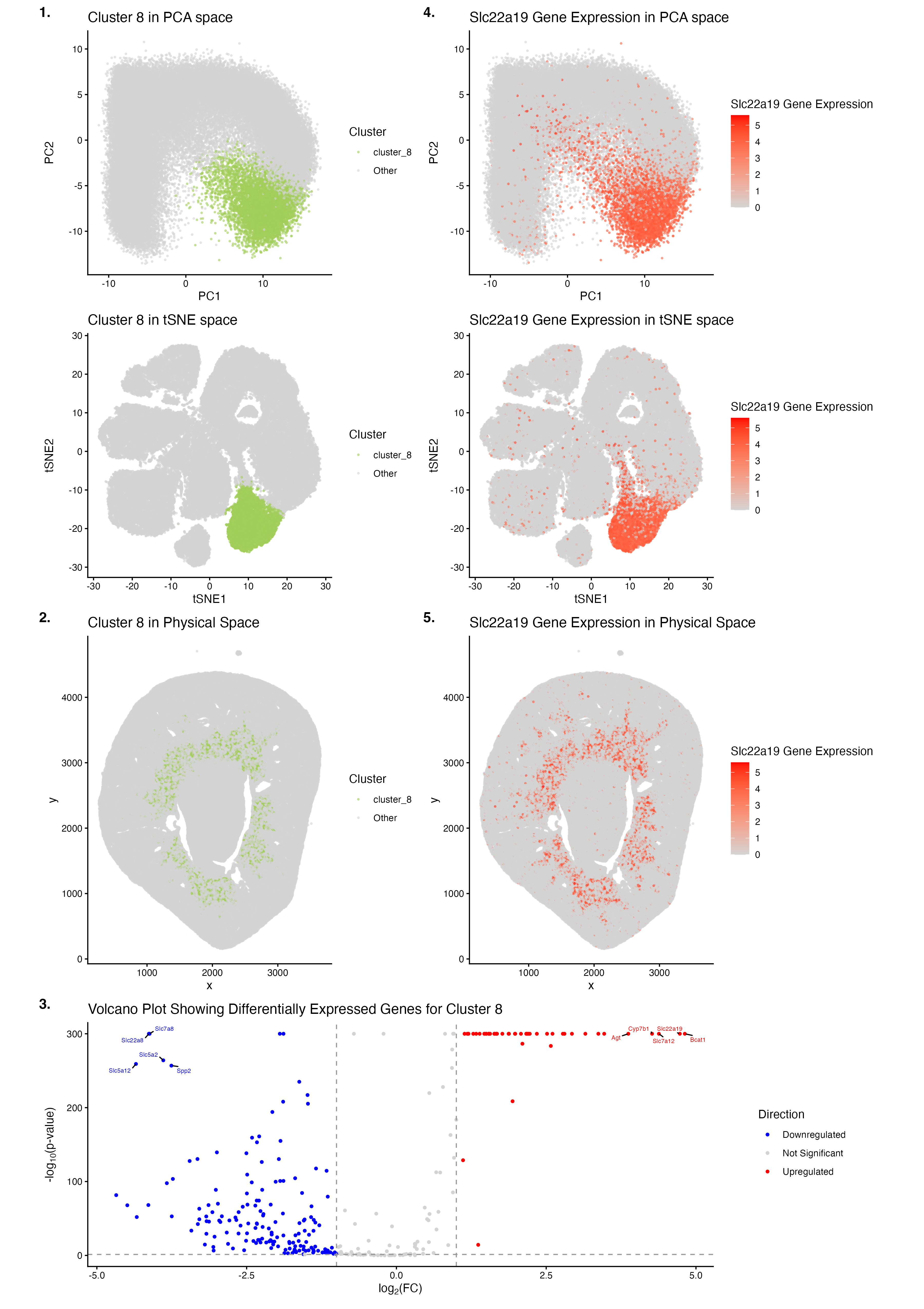
The figure identifies Cluster 8 as a coherent, transcriptionally distinct, and spatially localized cluster of cells in the Xenium data. K-means clustering was performed using k (centers) = 10, as this optimal value was the k at the elbow of the scree plot depicting total withinness on the y-axis and number of centroids k on the x-axis. Initial examination of the reduced dimensional space of PCA led to the selection of Cluster 8 as the cluster of interest, as it had minimal overlap with all of the remaining clusters and was distinctly congregated. In panel 1., Cluster 8 (olive green) was found to form a distinct cluster of cells in the linearly reduced dimensional space of PCA and the non-linearly reduced dimensional space of tSNE (light grey). In panel 2., Cluster 8 (olive green) was found to be concentrated in a spatially localized ring-like region, implying the marking of an anatomically organized compartment in the physical space (light grey). In panel 3., Cluster 8 shows its differentially expressed genes that are upregulated (red; e.g., Bcat1, Slc22a19, Slc7a12, Cyp7b1, Agt), not significantly changed in expression (light grey), or downregulated (blue; e.g., Slc22a8, Slc7a8, Slc5a12, Slc5a2, Spp2) compared to gene expressions in all of the remaining clusters. Given that Slc22a19 was found to be a differentially upregulated gene in Cluster 8 (pval = 1e-100, log2fc = 4.74521696) through the examination of outputs from the two-sided Wilcoxon rank-sum test performed to depict the volcano plot in panel 3., it was selected as a potential marker gene for Cluster 8. In panel 4., cells that highly express Slc22a19 (red) were found to form a distinct cluster in the linearly reduced dimensional space of PCA and the non-linearly reduced dimensional space of tSNE (light grey); these clusters also spatially co-localized to those formed by Cluster 8 in the PCA and tSNE spaces, respectively, indicating the Slc22a19 gene’s role as a marker gene for Cluster 8. In panel 5., cells that highly express Slc22a19 (red) were found to be concentrated in a spatially localized ring-like region, implying the marking of an anatomically organized compartment in the physical space (light grey); this ring-like region also spatially co-localized to that formed by Cluster 8 in the physical space, further validating the Slc22a19 gene’s role as a marker gene for Cluster 8.
Cluster 8 is speculated to correspond to proximal tubule epithelial cells. The Slc22a19 gene (encoding the organic anion transporter OAT5), upregulated in Cluster 8, has been characterized to be localized to the apical membrane of the S3 segment in renal proximal tubules, within mouse kidneys[1],[2],[3]. Moreover, the Agt gene (encoding angiotensinogen), also upregulated in Cluster 8, has been found to be synthesized at the S3 segment in renal proximal tubules[4],[5]. Additionally, the Slc7a12 (encoding asc-type amino acid transporter 2) and Cyp7b1 (encoding oxysterol 7-alpha-hydroxylase) genes, both upregulated in Cluster 8, have been characterized as female-biased and male-biased marker genes of the S3 segment in renal proximal tubules, respectively[6],[7]. Overall, the anatomical, ring-like localization of Cluster 8 in the mouse kidney, and references from the literature that discuss the roles of several highly upregulated gene markers for Cluster 8, strongly support that Cluster 8 corresponds to the cell-type identity of proximal tubule epithelial cells (most likely in the S3 segment).
[1] https://doi.org/10.14670/HH-25.1385
[2] https://doi.org/10.1152/ajprenal.00012.2004
[3] https://doi.org/10.1124/jpet.105.088583
[4] https://doi.org/10.1097/MNH.0b013e328359dbed
[5] https://doi.org/10.1111/j.1523-1755.2004.00635.x
[6] https://doi.org/10.1073/pnas.2026684118
[7] https://doi.org/10.1016/j.devcel.2019.10.005
Code
1
2
3
4
5
6
7
8
9
10
11
12
13
14
15
16
17
18
19
20
21
22
23
24
25
26
27
28
29
30
31
32
33
34
35
36
37
38
39
40
41
42
43
44
45
46
47
48
49
50
51
52
53
54
55
56
57
58
59
60
61
62
63
64
65
66
67
68
69
70
71
72
73
74
75
76
77
78
79
80
81
82
83
84
85
86
87
88
89
90
91
92
93
94
95
96
97
98
99
100
101
102
103
104
105
106
107
108
109
110
111
112
113
114
115
116
117
118
119
120
121
122
123
124
125
126
127
128
129
130
131
132
133
134
135
136
137
138
139
140
141
142
143
144
145
146
147
148
149
150
151
152
153
154
155
156
157
158
159
160
161
162
163
164
165
166
167
168
169
170
171
172
173
174
175
176
177
178
179
180
181
182
183
184
185
186
187
188
189
190
191
192
193
194
195
196
197
198
199
200
201
202
203
204
205
206
207
208
209
210
211
212
213
214
# Load the necessary libraries
library(ggplot2)
library(ggrepel)
library(patchwork)

# Read in data
data <- read.csv('~/Documents/genomic-data-visualization-2026/data/Xenium-IRI-ShamR_matrix.csv.gz')
pos <- data[,c('x', 'y')]
rownames(pos) <- data[,1]
gexp <- data[, 4:ncol(data)]
rownames(gexp) <- data[,1]

# Normalize
totgexp <- rowSums(gexp)
mat <- log10(gexp/totgexp * 1e6 + 1)

# PCA: linear dimensionality reduction
pcs <- prcomp(mat, center=TRUE, scale=FALSE)
plot(pcs$sdev[1:50]) # Scree plot: Will perform tSNE on top 10 PCs as it reaches the elbow of the graph

# tSNE: non-linear dimensionality reduction
set.seed(21126)
tsne <- Rtsne::Rtsne(pcs$x[, 1:10], dims=2, perplexity=30, verbose=TRUE)
emb <- tsne$Y
rownames(emb) <- rownames(mat)
colnames(emb) <- c('tSNE1', 'tSNE2')

# Determining the optimal k value for K-means clustering
totw <- sapply(2:25, function(k) {kmeans(pcs$x[,1:10], centers = k, nstart = 10, iter.max = 500, algorithm = "Lloyd")$tot.withinss})
df_totw <- data.frame(k = 2:25, tot.withinss = totw)
ggplot(df_totw, aes(x = k, y = tot.withinss)) + geom_point() + geom_line() + theme_test() # Scree plot: Optimal k = 10 found for K-means clustering

# K-means clustering
clusters <- as.factor(kmeans(pcs$x[,1:10], centers = 10)$cluster)
df_km <- data.frame(pcs$x, clusters)
ggplot(df_km, aes(x=PC1, y=PC2, col=clusters)) + geom_point(size = 0.5) # PC1 vs PC2: Selected cluster 8 as the one transcriptionally distinct cluster of cells

# Define labels for cluster 8 versus other clusters
cluster_label <- ifelse(clusters == 8, "cluster_8", "Other")

# Define colors for cluster 8 versus other clusters
cluster.cols <- c("Other" = "lightgrey", "cluster_8" = "darkolivegreen3")

# 1. Plot a panel visualizing cluster 8 in reduced dimensional space (PCA)
df_pca_cluster_8 <- data.frame(
  pcs$x,
  cluster = factor(cluster_label, levels = c("cluster_8", "Other"))
)
p1 <- ggplot(df_pca_cluster_8, aes(x = PC1, y = PC2, color = cluster)) +
  geom_point(size = 0.5, alpha = 0.5) +
  theme_classic() +
  scale_color_manual(values = cluster.cols) +
  labs(title = "Cluster 8 in PCA space",
       x = "PC1", y = "PC2", color = "Cluster")

# 1. Plot a panel visualizing cluster 8 in reduced dimensional space (tSNE)
df_tsne_cluster_8 <- data.frame(
  emb1 = emb[, 1],
  emb2 = emb[, 2],
  cluster = factor(cluster_label, levels = c("cluster_8", "Other"))
)
p2 <- ggplot(df_tsne_cluster_8, aes(x = emb1, y = emb2, color = cluster)) +
  geom_point(size = 0.5, alpha = 0.5) +
  theme_classic() +
  scale_color_manual(values = cluster.cols) +
  labs(title = "Cluster 8 in tSNE space",
       x = "tSNE1", y = "tSNE2", color = "Cluster")

# 2. Plot a panel visualizing cluster 8 in physical space
df_phys_cluster_8 <- data.frame(
  x = pos[, 1],
  y = pos[, 2],
  cluster = factor(cluster_label, levels = c("cluster_8", "Other"))
)
p3 <- ggplot(df_phys_cluster_8, aes(x = x, y = y, color = cluster)) +
  geom_point(size = 0.5, alpha = 0.5) +
  theme_classic() +
  scale_color_manual(values = cluster.cols) +
  coord_fixed() +
  labs(title = "Cluster 8 in Physical Space",
       x = "x", y = "y", color = "Cluster")

# Define cluster of interest
clusterofinterest <- clusters == "8"
othercells <- clusters != "8"

# Compute Wilcoxon p-values (two-sided for volcano plot)
pv <- sapply(colnames(mat), function(gene) {
  x1 <- mat[clusterofinterest, gene]
  x2 <- mat[othercells, gene]
  wilcox.test(x1, x2, alternative = "two.sided")$p.value
})
# Avoid p-values of zeros
pv[pv == 0] <- 1e-300

# Compute log2 fold-change
logfc <- sapply(colnames(mat), function(gene) {
  log2((mean(mat[clusterofinterest, gene]) + 1e-6) / (mean(mat[othercells, gene]) + 1e-6))
})

# 3. Plot a panel (volcano plot) visualizing differentially expressed genes for cluster 8
de <- data.frame(gene = colnames(mat), pval = pv, neglog10p = -log10(pv), log2fc = logfc)
de$status <- "Not Significant"
de$status[de$pval < 0.05 & de$log2fc > 1]  <- "Upregulated"
de$status[de$pval < 0.05 & de$log2fc < -1] <- "Downregulated"
p4 <- ggplot(de, aes(x = log2fc, y = neglog10p, color = status)) +
  geom_point(size = 1) +
  geom_vline(xintercept = c(-1, 1), linetype = "dashed", color = "grey60") +
  geom_hline(yintercept = -log10(0.05), linetype = "dashed", color = "grey60") +
  scale_color_manual(values = c("Downregulated" = "blue",
                                "Not Significant" = "lightgrey",
                                "Upregulated" = "red")) +
  theme_classic() +
  labs(
    title = "Volcano Plot Showing Differentially Expressed Genes for Cluster 8",
    x = expression("log"[2]*"(FC)"),
    y = expression("-log"[10]*"(p-value)"),
    color = "Direction"
  ) +
  geom_text_repel(
    data = subset(de, abs(log2fc) > 3.5 & neglog10p > 250),
    aes(label = gene),
    size = 2,
    max.overlaps = 20,
    show.legend = FALSE,
    segment.color = "black",
    segment.size = 0.5,
    min.segment.length = 0
  )

# Show top DE genes: selected Slc22a19 as a DE gene from this output (pval = 1e-100, log2fc = 4.74521696, status = Upregulated)
de[order(de$pval), ]

# 4. Plot a panel visualizing the Slc22a19 gene in reduced dimensional space (PCA)
df_pca_Slc22a19 <- data.frame(
  pcs$x,
  gene = mat[, 'Slc22a19']
)
p5 <- ggplot(df_pca_Slc22a19, aes(x = PC1, y = PC2, color = gene)) +
  geom_point(size = 0.5, alpha = 0.5) +
  theme_classic() +
  scale_color_gradient(low='lightgrey', high='red') +
  labs(
    title = "Slc22a19 Gene Expression in PCA space",
    x = "PC1", y = "PC2", color = "Slc22a19 Gene Expression"
  )

# 4. Plot a panel visualizing the Slc22a19 gene in reduced dimensional space (tSNE)
df_tsne_Slc22a19 <- data.frame(
  emb1 = emb[, 1],
  emb2 = emb[, 2],
  gene = mat[, 'Slc22a19']
)
p6 <- ggplot(df_tsne_Slc22a19, aes(x = emb1, y = emb2, color = gene)) +
  geom_point(size = 0.5, alpha = 0.5) +
  theme_classic() +
  scale_color_gradient(low='lightgrey', high='red') +
  labs(
    title = "Slc22a19 Gene Expression in tSNE space",
    x = "tSNE1", y = "tSNE2", color = "Slc22a19 Gene Expression"
  )

# 5. Plot a panel visualizing the Slc22a19 gene in physical space
df_phys_Slc22a19 <- data.frame(
  x = pos[, 1],
  y = pos[, 2],
  gene = mat[, 'Slc22a19']
)

p7 <- ggplot(df_phys_Slc22a19, aes(x = x, y = y, color = gene)) +
  geom_point(size = 0.5, alpha = 0.5) +
  theme_classic() +
  coord_fixed() +
  scale_color_gradient(low='lightgrey', high='red') +
  labs(
    title = "Slc22a19 Gene Expression in Physical Space",
    x = "x", y = "y", color = "Slc22a19 Gene Expression"
  )

# Plot all panels in one plot using patchwork
# Prompt to AI: "How do you code using the patchwork library so that the display of plots p1 to p7 is formatted in one p_all output plot
# with the following visual structure (plots p2 and p6 in the second row containing no numerical labels):
#(1.) p1     (4.) p5
#     p2          p6
#(2.) p3     (5.) p7
#(3.)       p4?"
p1_tag <- p1 + labs(tag = "1.")
p3_tag <- p3 + labs(tag = "2.")
p4_tag <- p4 + labs(tag = "3.")
p5_tag <- p5 + labs(tag = "4.")
p7_tag <- p7 + labs(tag = "5.")
tag_theme <- theme(
  plot.tag.position = c(0, 1),
  plot.tag = element_text(face = "bold")
)
p1_tag <- p1_tag + tag_theme
p3_tag <- p3_tag + tag_theme
p4_tag <- p4_tag + tag_theme
p5_tag <- p5_tag + tag_theme
p7_tag <- p7_tag + tag_theme
plot.layout <- "
AB
CD
EF
GG
"
p_all <-
  p1_tag + p5_tag +
  p2 + p6 +
  p3_tag + p7_tag +
  p4_tag +
  plot_layout(design = plot.layout)
p_all
ggsave("hw3_yhodo1.png", p_all, width = 12, height = 17, dpi = 300)