HW4-Identification and Characterization of a Transcriptionally Distinct Proximal Tubule Epithelial Cluster in Visium Kidney Spatial Transcriptomics Data

1. Describe your figure briefly.
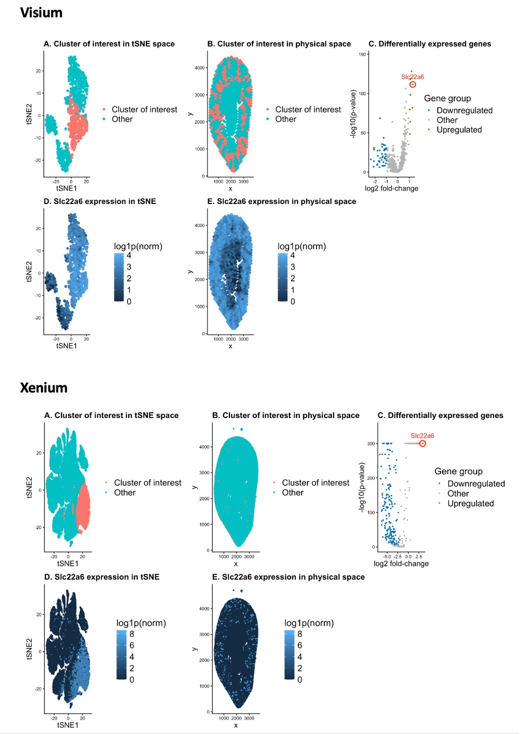
In these panels, I depict the Visium kidney spatial transcriptomics dataset in latent tSNE-embedded space and over the original spatial slide coordinates. Before clustering, I evaluated a range of k values (k = 2–20) by running k-means on the first 15 principal components and examining the total within-cluster sum of squares to identify an elbow point. This analysis suggested k = 10 for Xenium, which provides a reasonable balance between capturing transcriptional heterogeneity and avoiding over-fragmentation. In contrast, applying the same elbow-plot procedure to the Visium dataset suggested a smaller k (k = 5), consistent with the lower effective resolution and increased spot-level mixing in Visium.
In HW3 (Xenium), I originally aimed to identify an endothelial-like population using canonical endothelial markers (e.g., Kdr/VEGFR2, Pecam1, Cdh5, Vwf). However, upon inspection of the Visium gene set, Kdr was not present, and I did not detect other canonical endothelial marker genes in the available panel. Because this prevented a marker-based identification of endothelial cells in the Visium dataset, I instead began by identifying a different cell type in the Xenium.
Using k = 10 for Xenium, I examined the resulting clusters in tSNE-embedded space and selected a cluster of interest that forms a compact and well-separated group relative to surrounding clusters (A), indicating a transcriptionally distinct population. I then mapped the same cluster back onto the original spatial coordinates (B) to assess whether its spatial organization is biologically coherent rather than an artifact of the embedding.
Next, I performed differential expression analysis for the cluster of interest versus all other spots using a Wilcoxon rank-sum test and computed log2 fold change for each gene. Differential gene expression is visualized with a volcano plot (C), where genes are positioned by effect size (log2 fold change) and statistical significance (−log10 p-value). I selected Slc22a6, a gene supported by the Xenium panel, as a representative marker for the cluster of interest. Slc22a6 encodes the organic anion transporter OAT1 and is a well-established marker of proximal tubule epithelial cells[1].
I then visualized the normalized expression of Slc22a6 across the tSNE embedding (D) and across the original tissue coordinates (E). Enrichment of Slc22a6 within the selected cluster in latent space, together with a spatial distribution consistent with renal cortical proximal tubules, provides evidence that the cluster corresponds to a coherent population of proximal tubule epithelial cells.
Finally, having identified a robust, panel-supported proximal tubule marker and corresponding cell population in Xenium, I leveraged this information to guide interpretation in the Visium dataset. Differential expression analysis in Visium revealed Slc22a6 to be significantly upregulated, as evidenced by its prominent position in the Visium volcano plot. Visualization of Slc22a6 expression across the Visium latent embedding and physical tissue coordinates demonstrated a spatial pattern highly concordant with that observed in Xenium, with enrichment localized to cortical regions characteristic of proximal tubules. The close agreement in both transcriptional signature and physical spatial distribution across platforms supports the conclusion that the Visium cluster represents the same proximal tubule epithelial cell population identified in Xenium. This cross-platform strategy ensures that cell-type inference is driven by genes actually captured on each platform while maintaining a consistent and biologically coherent interpretation across datasets.
[1]Vávra, Jiří, et al. “Functional characterization of rare variants in OAT1/SLC22A6 and OAT3/SLC22A8 urate transporters identified in a gout and hyperuricemia cohort.” Cells 11.7 (2022): 1063.
2. Code (paste your code in between the ``` symbols)
1
2
3
4
5
6
7
8
9
10
11
12
13
14
15
16
17
18
19
20
21
22
23
24
25
26
27
28
29
30
31
32
33
34
35
36
37
38
39
40
41
42
43
44
45
46
47
48
49
50
51
52
53
54
55
56
57
58
59
60
61
62
63
64
65
66
67
68
69
70
71
72
73
74
75
76
77
78
79
80
81
82
83
84
85
86
87
88
89
90
91
92
93
94
95
96
97
98
99
100
101
102
103
104
105
106
107
108
109
110
111
112
113
114
115
116
117
118
119
120
121
122
123
124
125
126
127
128
129
130
131
132
133
134
135
136
137
138
139
140
141
142
143
144
145
146
147
148
149
150
151
152
153
154
155
156
157
158
159
160
161
162
163
164
165
166
167
168
169
170
171
172
173
174
175
176
177
178
179
180
181
182
183
184
185
186
187
188
189
190
191
192
193
194
195
196
197
198
199
200
201
202
203
204
205
206
207
208
209
210
211
212
213
214
215
216
217
218
219
220
221
222
223
224
225
226
227
228
229
230
231
232
233
234
235
236
237
238
239
240
241
242
243
244
245
246
247
248
249
250
251
252
253
254
255
256
257
258
259
260
261
262
263
264
265
266
267
268
269
270
271
272
273
274
275
276
277
278
279
280
281
282
283
284
285
286
287
288
289
290
291
## ---------------------------
## 0) Load required packages
## ---------------------------
pkgs <- c("data.table", "ggplot2", "patchwork", "Rtsne")

to_install <- pkgs[!pkgs %in% rownames(installed.packages())]
if (length(to_install) > 0) {
  install.packages(to_install, dependencies = TRUE)
}

library(data.table)
library(ggplot2)
library(patchwork)
library(Rtsne)


set.seed(123)

## ---------------------------
## 1) Load data
## ---------------------------
file <- "/Users/xl/Desktop/JHU2026Spring/Genomic-Data-Visualization/Homework/HW4/Visium-IRI-ShamR_matrix.csv.gz"
dt <- fread(file)

cat("Data dimensions:", dim(dt), "\n")

## 2) Explicitly set columns
barcode_col <- "V1"
x_col <- "x"
y_col <- "y"

stopifnot(all(c(barcode_col, x_col, y_col) %in% colnames(dt)))

barcodes <- dt[[barcode_col]]

pos <- data.frame(
  aligned_x = dt[[x_col]],
  aligned_y = dt[[y_col]]
)
rownames(pos) <- barcodes

## 3) Expression matrix: all remaining columns are genes
gene_cols <- setdiff(colnames(dt), c(barcode_col, x_col, y_col))

# Convert to numeric matrix safely
gexp_dt <- dt[, ..gene_cols]

for (cc in colnames(gexp_dt)) {
  if (!is.numeric(gexp_dt[[cc]])) {
    gexp_dt[[cc]] <- as.numeric(gexp_dt[[cc]])
  }
}

gexp <- as.matrix(gexp_dt)
rownames(gexp) <- barcodes

# Remove all-zero genes
gexp <- gexp[, colSums(gexp, na.rm = TRUE) > 0, drop = FALSE]

cat("Expression matrix dim:", dim(gexp), "\n")

## 4) Feature selection + normalization
topN <- 1500
gene_order <- order(colSums(gexp), decreasing = TRUE)
head(gene_order)
topgenes <- colnames(gexp)[gene_order[1:min(topN, ncol(gexp))]]
gsub <- gexp[, topgenes, drop = FALSE]

libsize <- rowSums(gsub)
libsize[libsize == 0] <- 1

norm <- (gsub / libsize) * 1e4
logexp <- log1p(norm)

## 5) PCA + kmeans
pcs <- prcomp(logexp, center = TRUE, scale. = TRUE)

ks <- 2:20

totw <- sapply(ks, function(k) {
  km_tmp <- kmeans(pcs$x[,1:15], centers = k, nstart = 20)
  km_tmp$tot.withinss
})

elbow_df <- data.frame(k = ks, tot_withinss = totw)

ggplot(elbow_df, aes(x = k, y = tot_withinss)) +
  geom_point(size = 2) +
  geom_line() +
  labs(title = "Elbow plot for choosing k",
       x = "Number of clusters (k)",
       y = "Total within-cluster sum of squares") +
  theme_classic()

k_final <- 5
km <- kmeans(pcs$x[, 1:15], centers = k_final, nstart = 25)
clusters <- km$cluster

pca_df <- data.frame(
  PC1 = pcs$x[,1],
  PC2 = pcs$x[,2],
  cluster = factor(clusters)
)

ggplot(pca_df, aes(PC1, PC2, color = cluster)) +
  geom_point(size = 0.6) +
  labs(title = "PCA of kidney Xenium data colored by k-means clusters",
       color = "Cluster") +
  theme_classic()


sp <- data.frame(pos)
sp$cluster <- factor(clusters)
ggplot(sp, aes(aligned_x, aligned_y)) +
  geom_point(size = 0.8, color = "steelblue") +
  facet_wrap(~ cluster, ncol = 3) +
  labs(title = "Spatial distribution of each cluster",
       x = "x", y = "y") +
  theme_classic()


## 6) Pick a cluster of interest
pca_xy <- pcs$x[, 1:2]
interest <- 3
cat("Cluster of interest:", interest, "\n")

cells_interest <- barcodes[clusters == interest]
cells_other <- barcodes[clusters != interest]

## 7) Differential expression (Wilcoxon)
wilcox_p <- sapply(colnames(logexp), function(g) {
  x <- logexp[cells_interest, g]
  y <- logexp[cells_other, g]
  suppressWarnings(wilcox.test(x, y)$p.value)
})


log2fc <- sapply(colnames(norm), function(g) {
  log2((mean(norm[cells_interest, g]) + 1e-3) /
         (mean(norm[cells_other, g]) + 1e-3))
})

de_df <- data.frame(
  gene = names(wilcox_p),
  pval = as.numeric(wilcox_p),
  neglog10p = -log10(as.numeric(wilcox_p) + 1e-300),
  log2fc = as.numeric(log2fc[names(wilcox_p)])
)

de_df <- de_df[order(de_df$pval, -de_df$log2fc), ]
ggplot(de_df, aes(x = log2fc, y = neglog10p)) +
  geom_point(size = 0.6) +
  geom_vline(xintercept = c(-1, 1), linetype = "dashed") +
  geom_hline(yintercept = -log10(1e-5), linetype = "dashed") +
  labs(title = "Volcano plot: cluster of interest vs others",
       x = "log2 fold-change",
       y = "-log10(p-value)") +
  theme_classic()

sig_up <- de_df[de_df$pval < 1e-5 & de_df$log2fc > 1, ]
head(sig_up, 20)


marker_gene <- "Slc22a6"


## 9) tSNE embedding
tsne_res <- Rtsne(pcs$x[, 1:15], perplexity = 30, check_duplicates = FALSE)
emb <- data.frame(tsne_res$Y)
colnames(emb) <- c("tSNE1","tSNE2")
colnames(emb)
head(emb)
emb$is_interest <- ifelse(clusters == interest, "Cluster of interest", "Other")

## 10) Panels
big_theme <- theme(
  plot.title  = element_text(size = 14, face = "bold"),
  legend.text = element_text(size = 15),
  legend.title = element_text(size = 16),
  axis.title  = element_text(size = 13),
  axis.text   = element_text(size = 8)
)

p1 <- ggplot(emb, aes(tSNE1, tSNE2, color = is_interest)) +
  geom_point(size = 1.5) +
  labs(title = "A. Cluster of interest in tSNE space", color = NULL) +
  theme_classic() +
  theme(
    legend.text = element_text(size = 13)
  ) +
  big_theme
sp <- data.frame(pos)
sp$is_interest <- ifelse(clusters == interest, "Cluster of interest", "Other")

p2 <- ggplot(sp, aes(aligned_x, aligned_y, color = is_interest)) +
  geom_point(size = 1.5) +
  labs(title = "B. Cluster of interest in physical space",
       x = "x", y = "y", color = NULL) +
  theme_classic() +
  theme(
    legend.text = element_text(size = 13)
  ) +
  big_theme

de_df$group <- "Other"
de_df$group[de_df$pval < 1e-5 & de_df$log2fc > 1]  <- "Upregulated"
de_df$group[de_df$pval < 1e-5 & de_df$log2fc < -1] <- "Downregulated"


de_df$label <- ""
de_df$label[de_df$gene == marker_gene] <- marker_gene
p3 <- ggplot(de_df, aes(log2fc, neglog10p, color = group)) +

  # normal points
  geom_point(size = 0.8) +

  # red circle highlight (no fill, just outline)
  geom_point(
    data = subset(de_df, gene == marker_gene),
    shape = 21,          # circle with border
    size = 4,
    stroke = 1.2,
    color = "red",
    fill = NA
  ) +

  # annotation text
  geom_text(
    data = subset(de_df, gene == marker_gene),
    aes(label = gene),
    color = "red",
    vjust = -1.2,
    size = 4,
    show.legend = FALSE
  ) +

  scale_color_manual(
    values = c(
      "Upregulated"   = "#D55E00",
      "Downregulated" = "#0072B2",
      "Other"         = "grey70"
    )
  ) +

  labs(
    title = "C. Differentially expressed genes",
    x = "log2 fold-change",
    y = "-log10(p-value)",
    color = "Gene group"
  ) +

  theme_classic() +
  big_theme +
  coord_cartesian(clip = "off") +
  scale_y_continuous(expand = expansion(mult = c(0.05, 0.2)))


emb$gene_expr <- logexp[, marker_gene]
p4 <- ggplot(emb, aes(tSNE1, tSNE2, color = gene_expr)) +
  geom_point(size = 1.5) +
  labs(title = paste("D.", marker_gene, "expression in tSNE"),
       color = "log1p(norm)") +
  theme_classic() +
  big_theme

sp$gene_expr <- logexp[, marker_gene]
p5 <- ggplot(sp, aes(aligned_x, aligned_y, color = gene_expr)) +
  geom_point(size = 1.5) +
  labs(title = paste("E.", marker_gene, "expression in physical space"),
       x = "x", y = "y", color = "log1p(norm)") +
  theme_classic() +
  big_theme


multi_panel <- wrap_plots(
  p1, p2, p3,
  p4, p5, plot_spacer(),
  ncol = 3, byrow = TRUE
)

ggsave(
  filename = "multi_panel_cluster_Slc22a6_Visium.png",
  plot = multi_panel,
  width = 12,
  height = 8,
  dpi = 300
)