HW4

Describe your figure briefly so we know what you are depicting (you no longer need to use precise data visualization terms as you have been doing). Write a description to convince me that your cluster interpretation is correct. Your description may reference papers and content that allowed you to interpret your cell cluster as a particular cell-type. You must provide attribution to external resources referenced. Links are fine; formatted references are not required. You must include the entire code you used to generate the figure so that it can be reproduced.
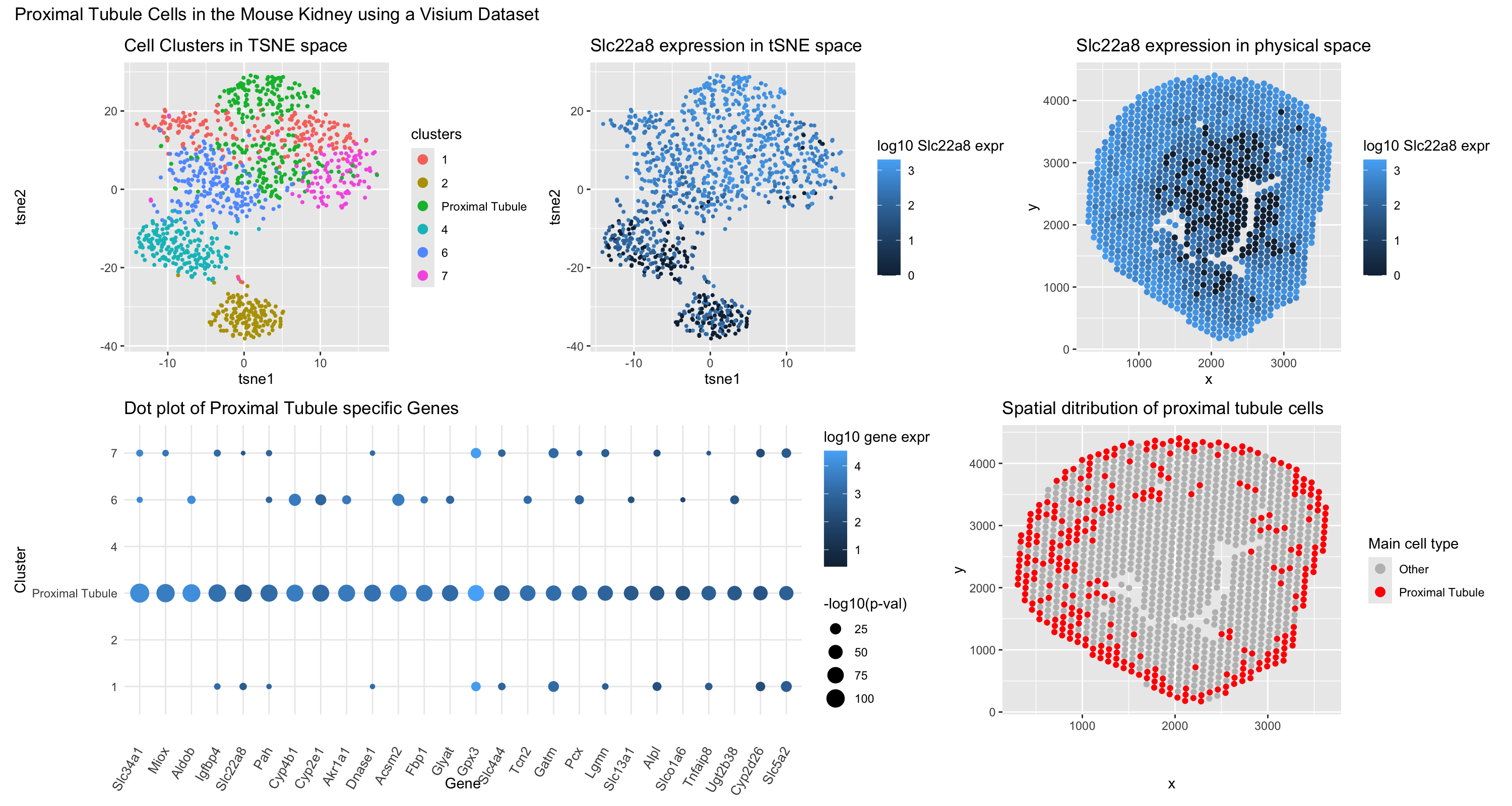
For this assignment, I replicated a data visualization aiming to identify proximal tubule cells in mouse kidneys, this time using the Visium dataset instead of the Xenium dataset. I employed the same set of plots as before. The top left panel shows cells projected into tSNE space with kmeans clustering (k=7) to distinguish the multiple cell types present in the mouse kidney. Upon analyzing these clusters, I found that both cluster 3 and cluster 5 highly expressed proximal tubule genes, so I combined and relabeled them accordingly. In the top middle panel, I used the Wilcox test to identify Slc22a8 as one of the most uniquely upregulated genes in the proximal tubule cluster and plotted its expression in tSNE space. The top right panel shows Slc22a8 expression mapped onto physical space. For the bottom left panel, I used the Wilcox test to identify a gene set that was both highly upregulated and statistically significant in the proximal tubule cluster, plotting expression as bubble color and significance as bubble size. Finally, the bottom right panel displays the spatial distribution of the cells I determined to be proximal tubule cells in physical space.
As before, I referenced a paper predicting seven distinct cell clusters in the kidney, excluding immune cells. Based on this, I applied k-means clustering with k=7 to differentiate cell types in the Visium dataset. However, as I began plotting the data, I noticed that many spots shared overlapping gene expression with known proximal tubule markers. This was expected because of the limited spatial resolution of sequencing based spatial transcriptomics. This led me to conclude that both cluster 3 and cluster 5 contained primarily proximal tubule cells, so I combined them into a single group. I then examined differentially upregulated genes in this combined cluster using an asymmetric Wilcox test, filtering for genes with a p-value below 1e-50. This allowed me to identify a set of genes most highly and significantly upregulated in the proximal tubule cluster. Finally, I corroborated this classification through literature searches, confirming that clusters 3 and 5 (renamed to “Proximal Tubule”) consisted primarily of proximal tubule cells.
Slc22a8 (OAT3) is an organic anion transporter highly expressed on the basolateral membrane of renal proximal tubule cells ((https://pmc.ncbi.nlm.nih.gov/articles/PMC6225997/)). In my data, Slc22a8 was one of the most differentially upregulated genes in the proximal tubule cluster and was chosen as the representative gene for the expression plots. A proteomic study of the kidney confirmed that SLC22A8 expression is restricted to the proximal tubule PLOS (https://journals.plos.org/plosone/article?id=10.1371/journal.pone.0116125).
Slc34a1 encodes the major sodium-phosphate cotransporter responsible for phosphate reabsorption in the kidney. It has been widely used as a definitive marker of fully differentiated proximal tubule epithelium ( https://www.pnas.org/doi/10.1073/pnas.1310653110).
Slc5a2 is a canonical proximal tubule marker that localizes to the brush border membrane of early proximal tubule segments. It is considered one of the most definitive markers for S1/S2 proximal tubule identity ( https://pmc.ncbi.nlm.nih.gov/articles/PMC3014039/). In my data, Slc5a2 was also highly specific to the proximal tubule cluster.
Slc4a4 encodes the electrogenic sodium bicarbonate cotransporter, which is expressed on the basolateral membrane of the proximal tubule in this nephron segment which was shown to be highly specific( https://www.frontiersin.org/journals/physiology/articles/10.3389/fphys.2013.00350/full).
Miox is a kidney-specific proximal tubule enzyme that catabolizes myo-inositol to d-glucuronic acid (https://pmc.ncbi.nlm.nih.gov/articles/PMC8977179/). Immunohistochemistry has localized MIOX specifically to proximal renal tubules, with no significant expression in other kideny regions. Its kidney-specific expression makes it a reliable proximal tubule marker.
In summary, the enrichment of these genes including solute transporters (Slc22a8, Slc34a1, Slc5a2, Slc4a4) and a kidney-specific metabolic enzyme (Miox) strongly supports the identification of clusters 3 and 5 as proximal tubule cells.
1
2
3
4
5
6
7
8
9
10
11
12
13
14
15
16
17
18
19
20
21
22
23
24
25
26
27
28
29
30
31
32
33
34
35
36
37
38
39
40
41
42
43
44
45
46
47
48
49
50
51
52
53
54
55
56
57
58
59
60
61
62
63
64
65
66
67
68
69
70
71
72
73
74
75
76
77
78
79
80
81
82
83
84
85
86
87
88
89
90
91
92
93
94
95
96
97
98
99
100
101
102
103
104
105
106
107
108
109
110
111
112
113
114
115
116
117
118
119
120
121
library(ggplot2)
library(Rtsne)
library(dplyr)
library(patchwork)
data <- read.csv('Visium-IRI-ShamR_matrix.csv.gz')
pos <- data [,c('x', 'y')]
rownames(pos) <- data[, 1]

gexp <- data[, 4:ncol(data)]
totgexp <- rowSums(gexp)
mat <- log10(gexp/totgexp * 10^6 + 1)
rownames(mat) <- data$X


## PCAs
pcs <- prcomp(mat, center=T, scale=F)
toppcs <- pcs$x[, 1:20]
tsne <- Rtsne::Rtsne(toppcs, dims = 2, perpexity = 30)
emb <- tsne$Y
rownames(emb) <- rownames(mat)
colnames(emb) <- c('tsne1', 'tsne2')


clusters <- as.factor(kmeans(toppcs, centers=7)$cluster)
names(clusters) <- rownames(mat)
df <- data.frame(emb, clusters, pos, pcs$x, gene=mat[ , 'Slc8a1'])

ggplot(df, aes(x = tsne1, y = tsne2, col = clusters)) + geom_point()
ggplot(df, aes(x = x, y = y, col = clusters)) + geom_point()
ggplot(df, aes(x = x, y = y, col = gene)) + geom_point()

vg <- apply(mat, 2, var)
vargenes <- names(sort(vg, decreasing=TRUE))
head(vargenes)

ggplot(df, aes(x=tsne1, y=tsne2, col=gene)) + geom_point()
ggplot(df, aes(x=tsne1, y=tsne2, col=clusters)) + geom_point()

clusterofinterest <- names(clusters)[clusters == 3 | clusters == 5]
othercells <- names(clusters)[clusters != 3 & clusters != 5]

out <- sapply(colnames(mat), function(gene) {
  x1 <- mat[clusterofinterest, gene]
  x2 <- mat[othercells, gene]
  wilcox.test(x1, x2, alternative='greater')$p.value
})
degs <- out[out < 1e-50]
degs <- sort(degs)
head(degs, 10)

proximal_tubule_genes <- c( "Spp2", "Slc7a8", "Slc6a19", "Slc5a2", "Slc5a12", 'Slc22a8', 'Slc34a1')
p <- list()
for(gene in proximal_tubule_genes){
  print(gene)
  df <- data.frame(emb, pos, clusters, gene=mat[,gene])
  p[[gene]] <- ggplot(df, aes(x=tsne1, y=tsne2, col=gene)) + geom_point() + labs(title = gene)
  print(p[[gene]])
}

levels(clusters)[levels(clusters) %in% c("3", "5")] <- "Proximal Tubule"

df <- data.frame(pos, emb, clusters)
gene <- 'Slc22a8'

gene_tsne <- ggplot(df, aes(x=tsne1, y=tsne2, col=mat[, gene])) + geom_point(size=0.75) +
  labs(title = paste(gene, 'expression in tSNE space'), color = paste('log10', gene, 'expr'))
gene_xy <- ggplot(df, aes(x=x, y=y, col=mat[, gene])) + geom_point() +
  labs(title = paste(gene, 'expression in physical space'), color = paste('log10', gene, 'expr'))
cluster_plot <- ggplot(df, aes(x=tsne1, y=tsne2, col=clusters)) + geom_point(size=0.75) +
  labs(title = 'Cell Clusters in TSNE space') + guides(color = guide_legend(override.aes = list(size = 3, alpha = 1)))
section_view <- ggplot(df, aes(x=x, y=y,
                               col = ifelse(clusters == "Proximal Tubule", "Proximal Tubule", "Other"))) +
  scale_color_manual(values = c("Proximal Tubule" = "red", "Other" = "grey")) +
  geom_point() +
  labs(title = 'Spatial ditribution of proximal tubule cells', color = 'Main cell type') +
  guides(color = guide_legend(override.aes = list(size = 3, alpha = 1)))

selected_genes <- names(degs)

avg <- sapply(selected_genes, function(g) tapply(mat[, g], clusters, mean, na.rm = TRUE))
avg_long <- as.data.frame(as.table(avg))
colnames(avg_long) <- c("cluster", "gene", "avg_expr")


sig_out <- data.frame(matrix(nrow = length(degs)))

for (cl in sort(unique(clusters))) {
  idx1 <- which(clusters == cl)
  idx2 <- which(clusters != cl)

  sig_out[cl] <- sapply(selected_genes, function(gene) {
    x1 <- mat[idx1, gene]
    x2 <- mat[idx2, gene]
    res <- wilcox.test(x1, x2, alternative='greater')$p.value
    -log10(res)
  })
}
rownames(sig_out) <- selected_genes

df_dot <- avg_long
df_dot$sig <- sapply(1:nrow(avg_long), function(i) {
  sig_out[avg_long$gene[i], as.character(avg_long$cluster[i])]
})
df_dot$sig[is.infinite(df_dot$sig)] <- max(df_dot$sig[is.finite(df_dot$sig)])

df_dot <- df_dot %>%
  group_by(gene) %>%
  filter(cluster[which.max(avg_expr)] == "Proximal Tubule") %>%
  ungroup()

dot_plot <- ggplot(df_dot, aes(x = gene, y = cluster)) +
  geom_point(aes(size = ifelse(sig >= 3, sig, NA), color = avg_expr )) +
  theme_minimal() +
  theme(axis.text.x = element_text(angle = 60, vjust = 0.5, hjust = 1, size = 10)) +
  labs(x = "Gene", y = "Cluster", color = "log10 gene expr", size = "-log10(p-val)", title = "Dot plot of Proximal Tubule specific Genes" )


(cluster_plot + gene_tsne + gene_xy) /
  (dot_plot + section_view + plot_layout(widths = c(2, 1))) +
  plot_annotation(title = "Proximal Tubule Cells in the Mouse Kidney using a Visium Dataset")