Identification of Thick Ascending Limb Cells in Xenium Dataset

Write a description to convince me you found the same cell-type. You will likely need to change your code from HW3. Write a description of what you changed and why you think you had to change it.
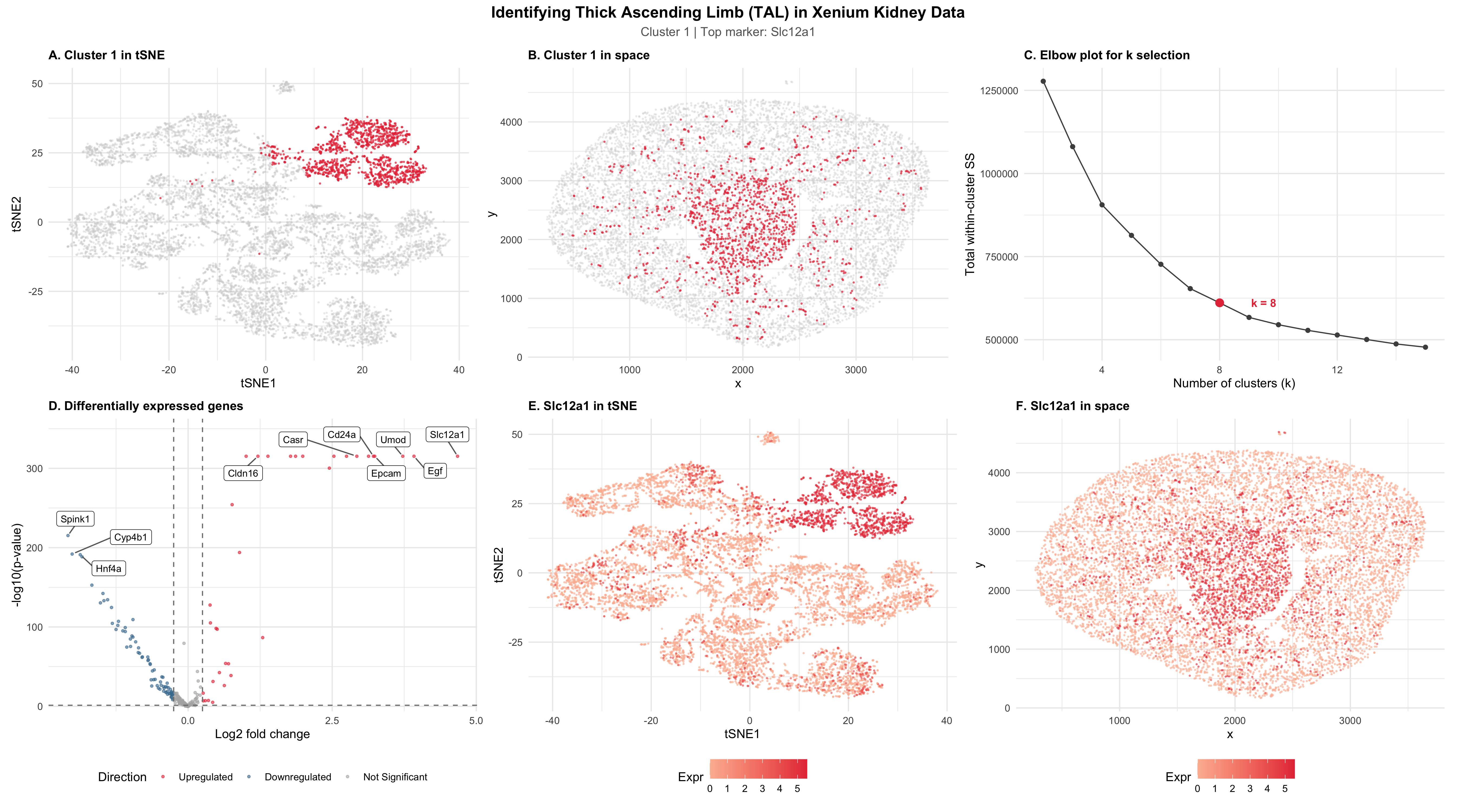
The visualization identifies Cluster 1 using k-means clustering (k = 8) on the Xenium kidney dataset as the same thick ascending limb (TAL) cell type that I identified as Cluster 5 in the Visium dataset for HW3. The gene expression was normalized using CPM and log10-transformed. Because the Xenium panel only contained 300 genes compared to the 20,000 in Visium, I used all genes directly for PCA without variable gene selection. tSNE was performed on the first 15 PCs, and I subsampled to 10,000 cells.
Panel C shows the elbow plot that was used to select k = 8, increased from k = 6 in HW3. This is because single-cell resolution in Xenium has more transcriptionally distinct populations than the Visium spots, which describe multiple cells. To identify the TAL cluster, I computed mean expression of Slc12a1 and Umod (the two TAL markers from HW3 present in the Xenium panel) across all clusters and selected Cluster 1, which had the highest expression of both by a wide margin.
Panels A and B show Cluster 1 highlighted in red in both the tSNE and physical space. The cluster forms a compact, well-separated group in the tSNE and localizes to the medulla region of the kidney. This is consistent with the TAL anatomy that matches the spatial localization of Cluster 5 in HW3.
Panel D is a bidirectional volcano plot showing upregulated genes in red and downregulated genes in blue from a two-sided Wilcoxon rank-sum test. The top upregulated genes that were identified included Slc12a1, Umod, Casr, Cldn16, Egf, Epcam, and Cd24a. The downregulated genes included Spink1 and Hnf4a, which are actually markers of other kidney cell types. As a result, this confirms cluster specificity.
Panels E and F show the Slc12a1 expression in both the tSNE and physical space, with cells sorted by expression so high-expressing cells are a darker shade of red than low-expressing cells. It can be seen in the panels that Slc12a1 is clearly higher in the Cluster 1 region for both of the views.
I interpret Cluster 1 as corresponding to the thick ascending limb (TAL) found in HW3 based on the convergence of multiple established TAL markers. First, Slc12a1 encodes the NKCC2 cotransporter, which is the defining TAL marker and the target of loop diuretics (https://www.genecards.org/cgi-bin/carddisp.pl?gene=SLC12A1). Umod encodes uromodulin, which is produced exclusively by TAL cells (https://www.proteinatlas.org/ENSG00000169344-UMOD). Additionally, Casr regulates paracellular calcium reabsorption along the TAL basolateral membrane (https://www.genecards.org/cgi-bin/carddisp.pl?gene=CASR). Lastly, Cldn16 mediates paracellular magnesium transport specifically in the TAL (https://www.genecards.org/cgi-bin/carddisp.pl?gene=CLDN16). These markers in addition to the medullary spatial localization confirms the same cell type as HW3.
You will likely need to change your code from HW3. Write a description of what you changed and why you think you had to change it.
-
I subsampled to 10,000 cells because the Xenium dataset contains 80,000 cells compared to only ~1,000 spots in the Visium dataset. Running PCA, tSNE, and k-means on the full dataset would likely be extremely slow or crash, so I subsampled to 10,000 cells following the approach that was demonstrated in class 6. This is enough cells to identify all the major cell populations.
-
In HW3 I selected the top 500 most variable genes from 20,000 to reduce noise and focus on informative features. The Xenium dataset only contains 300 genes total, which are focused on biologically relevant markers. Having to apply variable gene selection would discard important genes, so all the genes were used directly for PCA.
-
I increased k from 6 to 8 because each Visium spot captures a signal average over multiple cells, which blurs transcriptional boundaries between cell types and reduces the number of distinguishable clusters. In contrast, Xenium provides single-cell resolution, allowing me to pull more transcriptionally distinct populations. The addition of the elbow plot (Panel C) confirmed that k = 8 is appropriate, as total within-cluster SS shows diminishing returns beyond this point.
-
The TA noted that in HW3, my panels A and C (both tSNE) along with panels B and D (both physical space) were redundant because they showed overlapping information. One showed all clusters colored and one had only the cluster of interest highlighted. I addressed this by combining each view into a single panel, then plotted all other cells in grey and the cluster of interest in red.
-
The TA noted that Slc12a1 was not labeled in HW3’s volcano plot, weakening the connection between my chosen gene and the cluster. In the Xenium dataset, Slc12a1 is one of the top significantly upregulated genes for Cluster 1 and is prominently labeled on the volcano plot (Panel D), directly linking the featured gene to the DE analysis.
-
HW3’s volcano plot only highlighted upregulated genes, whereas examples in class showed bidirectionality. The updated version colors both upregulated genes in red and downregulated genes in blue. This provides a more complete picture of differential expression. The downregulated genes (Spink1, Hnf4a) are known markers of other kidney cell types, which further confirms the specificity of the TAL cluster.
Code
1
2
3
4
5
6
7
8
9
10
11
12
13
14
15
16
17
18
19
20
21
22
23
24
25
26
27
28
29
30
31
32
33
34
35
36
37
38
39
40
41
42
43
44
45
46
47
48
49
50
51
52
53
54
55
56
57
58
59
60
61
62
63
64
65
66
67
68
69
70
71
72
73
74
75
76
77
78
79
80
81
82
83
84
85
86
87
88
89
90
91
92
93
94
95
96
97
98
99
100
101
102
103
104
105
106
107
108
109
110
111
112
113
114
115
116
117
118
119
120
121
122
123
124
125
126
127
128
129
130
131
132
133
134
135
136
137
138
139
140
141
142
143
144
145
146
147
148
149
150
151
152
153
154
155
156
157
158
159
160
161
162
163
164
165
166
167
168
169
170
171
172
173
174
175
176
177
178
179
180
181
182
183
184
185
186
187
188
189
190
191
192
193
194
195
196
197
198
199
200
201
202
203
204
205
206
207
208
209
210
211
212
213
214
215
216
217
218
219
220
221
222
223
# LOAD DATA
setwd("/Users/emmameihofer/Documents/GitHub/genomic-data-visualization-2026")
data <- read.csv("data/Xenium-IRI-ShamR_matrix.csv.gz")
dim(data)

set.seed(42)
data <- data[sample(1:nrow(data), 10000), ]
dim(data)

pos <- data[, c('x', 'y')]
rownames(pos) <- data[, 1]
gexp <- data[, 4:ncol(data)]
rownames(gexp) <- data[, 1]

# CHECK FOR TAL MARKERS FROM HW3
tal_markers <- c('Slc12a1', 'Umod', 'Ppp1r1b', 'Nccrp1')
cat("TAL markers in Xenium panel:\n")
for (g in tal_markers) cat(g, ":", g %in% colnames(gexp), "\n")

# NORMALIZE
totgexp <- rowSums(gexp)
mat <- log10(gexp / totgexp * 1e6 + 1)

# PCA (all ~300 genes, no variable gene selection needed)
pcs <- prcomp(mat, center = TRUE, scale. = FALSE)

# tSNE
set.seed(42)
tsne <- Rtsne::Rtsne(pcs$x[, 1:15], dims = 2, perplexity = 30)
emb <- tsne$Y
rownames(emb) <- rownames(mat)
colnames(emb) <- c('tSNE1', 'tSNE2')

# K-MEANS CLUSTERING
# Compute elbow plot data
set.seed(42)
k_range <- 2:15
wss <- sapply(k_range, function(k) kmeans(pcs$x[, 1:15], centers = k, nstart = 10)$tot.withinss)
elbow_df <- data.frame(k = k_range, wss = wss)

# Choose k = 8
set.seed(42)
k <- 8
km <- kmeans(pcs$x[, 1:15], centers = k, nstart = 10)
clusters <- as.factor(km$cluster)

# IDENTIFY THE TAL CLUSTER
library(ggplot2)

available_markers <- tal_markers[tal_markers %in% colnames(mat)]
cat("\nAvailable TAL markers:", paste(available_markers, collapse = ", "), "\n")
if (length(available_markers) > 0) {
  for (g in available_markers) {
    cat("\nMean", g, "by cluster:\n")
    print(tapply(mat[, g], clusters, mean))
  }
}

# SET CLUSTER OF INTEREST
cluster_of_interest <- 1

# DIFFERENTIAL EXPRESSION
cells_in <- names(clusters)[clusters == cluster_of_interest]
cells_out <- names(clusters)[clusters != cluster_of_interest]

# Two-sided test to capture both up and downregulated genes
de_pvals_up <- sapply(colnames(mat), function(gene) {
  wilcox.test(mat[cells_in, gene], mat[cells_out, gene],
              alternative = 'greater')$p.value
})
de_pvals_down <- sapply(colnames(mat), function(gene) {
  wilcox.test(mat[cells_in, gene], mat[cells_out, gene],
              alternative = 'less')$p.value
})
de_pvals_twosided <- sapply(colnames(mat), function(gene) {
  wilcox.test(mat[cells_in, gene], mat[cells_out, gene],
              alternative = 'two.sided')$p.value
})

mean_in <- colMeans(mat[cells_in, , drop = FALSE])
mean_out <- colMeans(mat[cells_out, , drop = FALSE])
log2fc <- mean_in - mean_out

de_results <- data.frame(
  gene = names(de_pvals_twosided),
  pval = de_pvals_twosided,
  pval_up = de_pvals_up,
  pval_down = de_pvals_down,
  log2fc = log2fc,
  neglog10p = -log10(de_pvals_twosided)
)

# LLM Prompt:  What can I do to prevent the visualization labels from being cut off at the top
# Cap Inf values in neglog10p (from p-values of exactly 0)
max_finite <- max(de_results$neglog10p[is.finite(de_results$neglog10p)])
de_results$neglog10p[is.infinite(de_results$neglog10p)] <- max_finite * 1.05

de_results <- de_results[order(de_results$pval), ]

cat("\nTop 20 upregulated genes:\n")
print(head(de_results[order(de_results$pval_up), ], 20))

# SELECT TOP GENE
top_gene <- "Slc12a1"
cat("\nTop marker gene:", top_gene, "\n")

# MULTI-PANEL FIGURE
library(patchwork)
library(ggrepel)

cluster_highlight <- ifelse(clusters == cluster_of_interest,
                            paste0("Cluster ", cluster_of_interest), "Other")
cluster_highlight <- factor(cluster_highlight,
                            levels = c(paste0("Cluster ", cluster_of_interest), "Other"))

df <- data.frame(pos, emb, cluster = clusters,
                 cluster_highlight = cluster_highlight,
                 top_gene_expr = mat[, top_gene])
df_other <- df[df$cluster_highlight == "Other", ]
df_coi <- df[df$cluster_highlight != "Other", ]

theme_hw <- theme_minimal(base_size = 11) +
  theme(plot.title = element_text(face = "bold", size = 11),
        legend.position = "bottom",
        plot.margin = margin(5, 10, 5, 5))

# Panel A: Cluster highlighted in tSNE
pA <- ggplot() +
  geom_point(data = df_other, aes(x = tSNE1, y = tSNE2),
             color = "#D3D3D3", size = 0.3, alpha = 0.3) +
  geom_point(data = df_coi, aes(x = tSNE1, y = tSNE2),
             color = "#E63946", size = 0.3, alpha = 0.6) +
  labs(title = paste0("A. Cluster ", cluster_of_interest, " in tSNE"),
       x = "tSNE1", y = "tSNE2") +
  theme_hw + theme(legend.position = "none")

# Panel B: Cluster highlighted in physical space
pB <- ggplot() +
  geom_point(data = df_other, aes(x = x, y = y),
             color = "#D3D3D3", size = 0.3, alpha = 0.3) +
  geom_point(data = df_coi, aes(x = x, y = y),
             color = "#E63946", size = 0.3, alpha = 0.6) +
  labs(title = paste0("B. Cluster ", cluster_of_interest, " in space"),
       x = "x", y = "y") +
  theme_hw + theme(legend.position = "none")

# Panel C: Elbow plot for k justification
pC <- ggplot(elbow_df, aes(x = k, y = wss)) +
  geom_line(color = "grey30") +
  geom_point(size = 1.5, color = "grey30") +
  geom_point(data = elbow_df[elbow_df$k == 8, ], aes(x = k, y = wss),
             color = "#E63946", size = 3) +
  annotate("text", x = 9.5, y = elbow_df$wss[elbow_df$k == 8],
           label = "k = 8", color = "#E63946", fontface = "bold", size = 3.5) +
  labs(title = "C. Elbow plot for k selection",
       x = "Number of clusters (k)", y = "Total within-cluster SS") +
  theme_hw + theme(legend.position = "none")

# Panel D: Bidirectional volcano plot
de_results$direction <- ifelse(de_results$pval < 0.05 & de_results$log2fc > 0.25, "Upregulated",
                        ifelse(de_results$pval < 0.05 & de_results$log2fc < -0.25, "Downregulated",
                        "Not Significant"))
de_results$direction <- factor(de_results$direction,
                               levels = c("Upregulated", "Downregulated", "Not Significant"))

# Label top 5 upregulated + top 3 downregulated + TAL markers
top5_up <- head(de_results$gene[de_results$direction == "Upregulated"], 5)
top3_down <- head(de_results$gene[de_results$direction == "Downregulated"], 3)
label_genes <- unique(c(top5_up, top3_down, available_markers))
de_results$label <- ifelse(de_results$gene %in% label_genes, de_results$gene, "")

volcano_cols <- c("Upregulated" = "#E63946", "Downregulated" = "#457B9D", "Not Significant" = "grey70")

pD <- ggplot(de_results, aes(x = log2fc, y = neglog10p)) +
  geom_point(aes(col = direction), size = 0.8, alpha = 0.6) +
  scale_color_manual(values = volcano_cols) +
  geom_label_repel(aes(label = label), size = 3, max.overlaps = 20,
                   box.padding = 0.5, point.padding = 0.3,
                   min.segment.length = 0, segment.color = "grey40",
                   fill = "white", label.size = 0.2) +
  geom_hline(yintercept = -log10(0.05), linetype = "dashed", color = "grey50") +
  geom_vline(xintercept = c(-0.25, 0.25), linetype = "dashed", color = "grey50") +
  scale_y_continuous(expand = expansion(mult = c(0.02, 0.15))) +
  labs(title = "D. Differentially expressed genes",
       x = "Log2 fold change", y = "-log10(p-value)", color = "Direction") +
  theme_hw

# Sort so high-expression cells drawn on top
df_sorted <- df[order(df$top_gene_expr), ]

# Panel E: Top gene in tSNE
pE <- ggplot(df_sorted, aes(x = tSNE1, y = tSNE2, col = top_gene_expr)) +
  geom_point(size = 0.3, alpha = 0.5) +
  scale_color_gradient2(low = "grey90", mid = "#FCBBA1", high = "#E63946",
                        midpoint = median(df$top_gene_expr)) +
  labs(title = paste0("E. ", top_gene, " in tSNE"), color = "Expr") +
  theme_hw

# Panel F: Top gene in physical space
pF <- ggplot(df_sorted, aes(x = x, y = y, col = top_gene_expr)) +
  geom_point(size = 0.3, alpha = 0.5) +
  scale_color_gradient2(low = "grey90", mid = "#FCBBA1", high = "#E63946",
                        midpoint = median(df$top_gene_expr)) +
  labs(title = paste0("F. ", top_gene, " in space"), color = "Expr") +
  theme_hw

# ASSEMBLE AND SAVE
# Layout: 2 rows of 3
top_row <- pA + pB + pC + plot_layout(nrow = 1)
bot_row <- pD + pE + pF + plot_layout(nrow = 1)

final_fig <- (top_row / bot_row) +
  plot_annotation(
    title = 'Identifying Thick Ascending Limb (TAL) in Xenium Kidney Data',
    subtitle = paste0('Cluster ', cluster_of_interest, ' | Top marker: ', top_gene),
    theme = theme(
      plot.title = element_text(face = "bold", size = 14, hjust = 0.5),
      plot.subtitle = element_text(size = 11, hjust = 0.5, color = "grey40")
    )
  )

ggsave('hw4_figure.png', final_fig, width = 18, height = 10, dpi = 300, bg = "white")
ggsave("~/Downloads/emeihof1_HW4.png", final_fig, width = 18, height = 10, dpi = 300, bg = "white")