HW 5

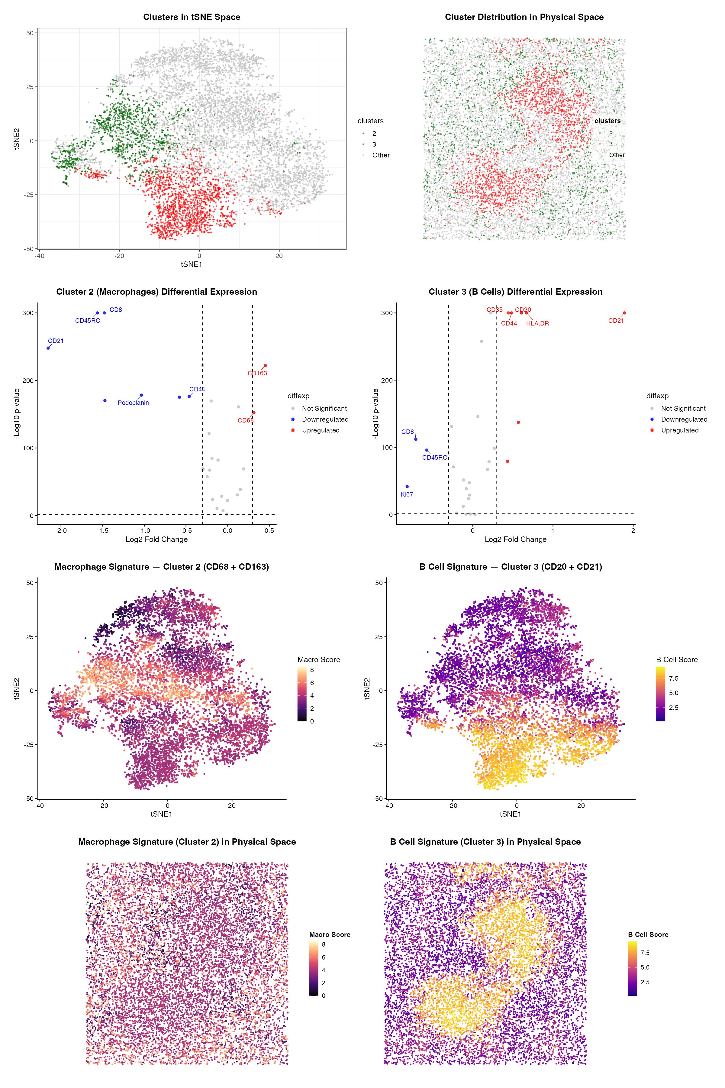
###Summary To identify the tissue structure represented in this CODEX dataset, I performed quality control, dimensionality reduction, k means clustering, differential expression analysis, and cell-type signature scoring. Proteins with low total expression (summed counts < 1000) were filtered out, and the remaining protein intensities were log-normalized. PCA was applied to reduce dimensionality, followed by tSNE visualization using the top 20 PCs. An elbow plot determined k=7 and K means clustering was done. I identified and characterized Cluster 2 and Cluster 3. ###Cell Type 1: Macrophages (Cluster 2) Cluster 2 shows upregulation of CD68 and CD163, two canonical macrophage markers. CD68 is a transmembrane glycoprotein highly expressed in tissue macrophages and is widely used as a macrophage marker. CD163 is a scavenger receptor expressed specifically on immunosuppressive M2-polarized macrophages. They are typically found in tissue involved in phagocytosis of red blood cells. In physical space, macrophage are distributed across the tissue, consistent with the red pulp of the spleen. In red pulp, resident macrophages (particularly CD163) are densely packed and responsible for filtering senescent erythrocytes from circulation. ###Cell Type 2: B Cells (Cluster 3) Cluster 3 shows upregulation of CD20, CD21, CD44, and HLA-DR. CD20 is a well-established B cell surface marker. CD21 is expressed on B cells and plays a key role in enhancing B cell receptor signaling by binding antigens. In physical space, the B cell signature score is strikingly localized to a discrete, dense circular region. This is clearly a hallmark of a lymphoid follicle or white pulp nodule. ###Tissue Identity: White Pulp of the Spleen The co-occurrence of a spatially confined, CD20/CD21 B cell population organized into a focal nodular structure indicated white pulp of the spleen. Also, CD68/CD163 (macrophage population) was broadly distributed which again is most consistent with the white pulp of the spleen. The white pulp is organized into B cell follicles surrounded by red pulp, which is enriched by red pulp macrophages. This interpretation is supported by splenic architecture, in which follicular B cells expressing CD21 and CD20 are spatially separated from the macrophage-rich red pulp that handles erythrocyte clearance. ###References https://pmc.ncbi.nlm.nih.gov/articles/PMC4479725/ https://pmc.ncbi.nlm.nih.gov/articles/PMC3439854/ https://www.proteinatlas.org/ENSG00000204287-HLA-DRA https://www.proteinatlas.org/ENSG00000117322-CR2 https://www.proteinatlas.org/ENSG00000156738-MS4A1 https://www.proteinatlas.org/ENSG00000129226-CD68 https://www.proteinatlas.org/ENSG00000177575-CD163
1
2
3
4
5
6
7
8
9
10
11
12
13
14
15
16
17
18
19
20
21
22
23
24
25
26
27
28
29
30
31
32
33
34
35
36
37
38
39
40
41
42
43
44
45
46
47
48
49
50
51
52
53
54
55
56
57
58
59
60
61
62
63
64
65
66
67
68
69
70
71
72
73
74
75
76
77
78
79
80
81
82
83
84
85
86
87
88
89
90
91
92
93
94
95
96
97
98
99
100
101
102
103
104
105
106
107
108
109
110
111
112
113
114
115
116
117
118
119
120
121
122
123
124
125
126
127
128
129
130
131
132
133
134
135
136
137
138
139
140
141
142
143
144
145
146
147
148
149
150
151
152
153
154
155
156
157
158
159
160
161
162
163
164
165
166
167
168
169
170
171
172
173
174
175
176
177
178
179
180
181
182
183
184
185
186
187
188
189
190
191
192
193
194
195
196
197
198
199
200
201
202
203
204
205
206
207
208
209
210
211
212
213
214
215
216
217
218
219
220
221
codex_data <- read.csv("~/Desktop/codex_spleen2.csv.gz")

library(ggplot2)
library(patchwork)
library(Rtsne)
library(ggrepel)
library(dplyr)
library(cluster)
library(reshape2)

codex_data <- read.csv("~/Desktop/codex_spleen2.csv.gz")
spatial_coords <- codex_data[, 2:3]
colnames(spatial_coords) <- c("x", "y")

cell_area    <- codex_data[, 4]
protein_data <- codex_data[, 5:ncol(codex_data)]

protein_data_filter <- protein_data[, colSums(protein_data) > 1000]
protein_data_norm <- log1p(protein_data_filter)

##elbow plot
wss <- sapply(1:10, function(k) {kmeans(protein_data_norm, centers = k, nstart = 10)$tot.withinss})

## k means, i chose k=7
set.seed(0)
kmeans_result <- kmeans(protein_data_norm, centers = 7)
full_labels <- as.character(kmeans_result$cluster)

clusters <- as.character(kmeans_result$cluster)
keep_clusters <- c("3", "2")
clusters[!clusters %in% keep_clusters] <- "Other"
clusters <- as.factor(clusters)

##PCA + tSNE
pcs <- prcomp(protein_data_norm, scale. = TRUE)
set.seed(0)
tsne_result <- Rtsne(pcs$x[, 1:20], perplexity = 30, check_duplicates = FALSE)
tsne_df <- data.frame(tsne_result$Y, clusters)
colnames(tsne_df) <- c("tSNE1", "tSNE2", "clusters")
pos_df <- data.frame(spatial_coords, clusters)

##cluster plots
cluster_colors <- c("Other" = "grey",
                    "3" = "red",
                    "2" = "darkgreen")
cluster_colors_light <- c("Other" = "grey",
                          "3" = "red",
                          "2" = "darkgreen")

## in tSNE space
p1 <- ggplot(tsne_df, aes(x = tSNE1, y = tSNE2, color = clusters)) +
  geom_point(alpha = 0.5, size = 0.5) +
  scale_color_manual(values = cluster_colors) +
  theme_bw(base_size = base_size) + theme_panel +
  labs(title = "Clusters in tSNE Space")

## in physical space
p2 <- ggplot(pos_df, aes(x = x, y = y, color = clusters)) +
  geom_point(size = 0.4, alpha = 0.5) +
  scale_color_manual(values = cluster_colors_light) +
  coord_fixed() +
  theme_bw(base_size = base_size) +
  theme_spatial +
  labs(title = "Cluster Distribution in Physical Space")

##DIFFERENTIAL EXPRESSION
## AI prompt: can you help me find the differential expression in cluster 2 and 3. make a volcano plot with upregulated, downregulated, not significant. also, use the log scale
  run_diffexp <- function(protein_norm,
                          cluster_label,
                          clusters_vec) {
    in_clust  <- clusters_vec == cluster_label
    out_clust <- clusters_vec != cluster_label
    pv <- sapply(colnames(protein_norm), function(i) {
      wilcox.test(protein_norm[in_clust, i], protein_norm[out_clust, i])$p.value
    })
    logfc <- sapply(colnames(protein_norm), function(i) {
      log2(mean(protein_norm[in_clust, i]) / mean(protein_norm[out_clust, i]))
    })

    df <- data.frame(
      gene = colnames(protein_norm),
      logfc = logfc,
      logpv = -log10(pv + 1e-300)
    )
    df$diffexp <- "Not Significant"
    df$diffexp[df$logpv > 1.3 & df$logfc >  0.3] <- "Upregulated"
    df$diffexp[df$logpv > 1.3 & df$logfc < -0.3] <- "Downregulated"
    df$diffexp <- factor(df$diffexp,
                         levels = c("Not Significant", "Downregulated", "Upregulated"))
    df
  }

  make_volcano <- function(df, title) {
    labeled <- bind_rows(
      df %>% filter(diffexp == "Upregulated")   %>% arrange(desc(logpv)) %>% head(5),
      df %>% filter(diffexp == "Downregulated") %>% arrange(desc(logpv)) %>% head(5)
    )

    ggplot(df, aes(logfc, logpv, color = diffexp)) +
      geom_point(alpha = 0.8) +
      geom_vline(xintercept = c(-0.3, 0.3), linetype = "dashed") +
      geom_hline(yintercept = 1.3, linetype = "dashed") +
      geom_text_repel(
        data = labeled,
        aes(label = gene),
        size = 3.5,
        max.overlaps = 20,
        box.padding = 0.5,
        segment.size = 0.3
      ) +
      scale_color_manual(values = c(
        "Downregulated" = "blue",
        "Not Significant" = "grey",
        "Upregulated" = "red"
      )) +
      theme_classic(base_size = base_size) +
      theme_panel +
      labs(title = title, x = "Log2 Fold Change", y = "-Log10 p-value")
  }

  df_c1 <- run_diffexp(protein_data_norm, "2", full_labels)
  df_c4 <- run_diffexp(protein_data_norm, "3", full_labels)

  p3 <- make_volcano(df_c1, "Cluster 2 (Macrophages) Differential Expression")
  p4 <- make_volcano(df_c4, "Cluster 3 (B Cells) Differential Expression")

  #SIGNATURE SCORES
  bcell_markers <- intersect(c("CD20", "CD21"), colnames(protein_data_norm))
  macro_markers <- intersect(c("CD68", "CD163"), colnames(protein_data_norm))

  tsne_df$Bcell_score <- rowMeans(protein_data_norm[, bcell_markers, drop = FALSE])
  tsne_df$Macro_score <- rowMeans(protein_data_norm[, macro_markers, drop = FALSE])

  pos_df$Bcell_score  <- rowMeans(protein_data_norm[, bcell_markers, drop = FALSE])
  pos_df$Macro_score  <- rowMeans(protein_data_norm[, macro_markers, drop = FALSE])

  #B cell in tsne
  p5 <- ggplot(tsne_df, aes(tSNE1, tSNE2, color = Bcell_score)) +
    geom_point(size = 0.7) +
    scale_color_viridis_c(option = "plasma", name = "B Cell Score") +
    theme_classic(base_size = base_size) +
    theme_panel +
    guides(color = guide_colorbar(
      barwidth = 1,
      barheight = 6,
      title.position = "top"
    )) +
    labs(title = "B Cell Signature — Cluster 3 (CD20 + CD21)")

  #Macrophage in tsne
  p7 <- ggplot(tsne_df, aes(tSNE1, tSNE2, color = Macro_score)) +
    geom_point(size = 0.7) +
    scale_color_viridis_c(option = "magma", name = "Macro Score") +
    theme_classic(base_size = base_size) +
    theme_panel +
    guides(color = guide_colorbar(
      barwidth = 1,
      barheight = 6,
      title.position = "top"
    )) +
    labs(title = "Macrophage Signature — Cluster 2 (CD68 + CD163)")

  #B cell in physical
  p6 <- ggplot(pos_df, aes(
    x = x, y = y, color = Bcell_score
  )) +
    geom_point(size = 0.5) +
    scale_color_viridis_c(option = "plasma", name = "B Cell Score") +
    coord_fixed() +
    theme_bw(base_size = base_size) +
    theme_spatial +
    guides(
      color = guide_colorbar(
        barwidth = 1,
        barheight = 6,
        title.position = "top",
        position = "right"
      )
    ) +
    labs(title = "B Cell Signature (Cluster 3) in Physical Space")

  #Macrophage in physical
  p8 <- ggplot(pos_df, aes(
    x = x, y = y, color = Macro_score
  )) +
    geom_point(size = 0.5) +
    scale_color_viridis_c(
      option = "magma",
      name = "Macro Score",
      position = "right"
    ) +
    coord_fixed() +
    theme_bw(base_size = base_size) +
    theme_spatial +
    guides(
      color = guide_colorbar(
        barwidth = 1,
        barheight = 6,
        title.position = "top",
        position = "right"
      )
    ) +
    labs(title = "Macrophage Signature (Cluster 2) in Physical Space")

  ## final plot
  final_plot <- (p1 | p2) /
    (p3 | p4) /
    (p7 | p5) /
    (p8 | p6) +
    plot_layout(heights = c(1, 1, 1, 1))
##help from AI: save this without causing overlaps between plots or even in the same plot
  ggsave(
    "~/Desktop/codex_final_plot_v2.png",
    plot   = final_plot,
    width  = 16,
    height = 24,
    dpi    = 150
  )

  final_plot