Validating Identity of Splenic White Pulp with B-cell and T-cell Markers

The CODEX dataset for spleen tissue was analyzed in this visualization. To identify a tissue structure in the data, a combination of methods were utilized such as normalization, PCA and tSNE dimensionality reduction, k-means clustering, and differential expression analysis with Wilcoxon rank-sum tests.
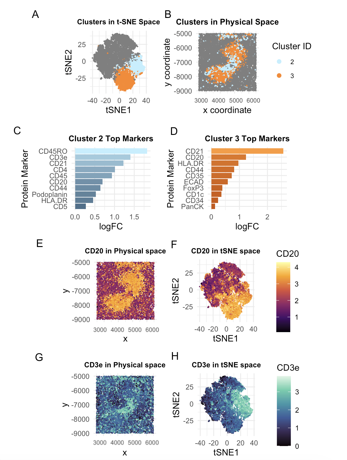
To start off with, distribution of total protein expression and area was assessed via a histogram, where data appeared right skewed. Hence, it was normalized and log transformed. Next, PCA was performed and with a scree plot, I decided that the first 25 pcs captured >90% of the variance. Total withiness for deciding k clusters was calculated and the elbow plot showed a bend at k = 6. This optimal k was validated by plotting the clusters in tSNE space (Panel A). Clusters were plotted in Physical space as well (Panel B). Clusters 2 and 3 stood out to me due to their spatially distinct presence in the tSNE space but anatomical relationship in the physical space, with both clusters encompassing a central area of the tissue being analyzed, leading me to hypothesize they may be part of the same tissue structure. These two clusters were colored in contrasting hues (orange for Cluster 3 and light blue for Cluster 2) and highlighted in both Panels A and B. This color scheme follows through the entire visualization, with Panels C, G, H maintaining blue hues representing Cluster 2 and panels D, E, F maintaining orange hues representing Cluster 3.
In panels C and D, protein expression profiles for respective clusters were analyzed by the top 10 differentially expressed markers being plotted based on their log fold change values. CD45RO and CD3e were the top 2 expressed markers for cluster 2. CD21 and CD20 were the top 2 expressed for cluster 3. Based on literature, CD45RO is a marker for memory T cells and CD3e is a T-cell surface marker. This indicates that cluster 3 is characterized by a significant T-cell population. As for Cluster 2, both CD20 and CD21 are B-cell markers, with CD21 specifically being expressed on mature B cells and Follicular Dendritic Cells (FDC).
When the T-cell marker CD3e was plotted in tSNE and Physical space (Panel G and H), it is clear that expression is localized to Cluster 2. As for B-cell marker CD20, we see the highest expression in Cluster 3 but we also see increased expression in Cluster 2, as further confirmed by CD20 being present in both Panels C and D as one of the top 10 DE genes. This is because CD20+ T cells do make up a subset of CD3+ T cells as well.
As for connecting this information to the spleen, Cluster 2’s B-cell and FDC enriched regions indicate B-cell follicles, which are only located in the white pulp. These follicles surround a T-cell rich zone called the periarteriolar lymphatic sheath (PALS), which is very likely to be cluster 3. This information is supported by our spatial plots which show Cluster 3 encompassing Cluster 2. To convince you even further, we do not see endothelial markers such as CD31 and CD34 which would indicate arteries/veins. Nor do we see key macrophage markers of the red pulp such as CD68 and CD163. Lastly, Capsule/trabeculae would exhibit collagen markers such as SMA. Since these markers are not prominent through our Wilcoxon tests, we are again led to the conclusion Clusters 2 and 3 are visualized the white pulp.
A general note is that Panels A-B, E-F, G-H share legends, so only one is displayed to avoid redundancy.
References:
-
https://www.nature.com/articles/s41598-017-11122
-
https://www.ncbi.nlm.nih.gov/gene/916
-
https://pmc.ncbi.nlm.nih.gov/articles/PMC7271567/
-
https://www.pathologyoutlines.com/topic/cdmarkerscd21.html
-
https://www.nature.com/articles/s41598-021-00007-0
-
https://rupress.org/jem/article-abstract/187/7/997/7563/The-Sequential-Role-of-B-Cells
Code
1
2
3
4
5
6
7
8
9
10
11
12
13
14
15
16
17
18
19
20
21
22
23
24
25
26
27
28
29
30
31
32
33
34
35
36
37
38
39
40
41
42
43
44
45
46
47
48
49
50
51
52
53
54
55
56
57
58
59
60
61
62
63
64
65
66
67
68
69
70
71
72
73
74
75
76
77
78
79
80
81
82
83
84
85
86
87
88
89
90
91
92
93
94
95
96
97
98
99
100
101
102
103
104
105
106
107
108
109
110
111
112
113
114
115
116
117
118
119
120
121
122
123
124
125
126
127
128
129
130
131
132
133
134
135
136
137
138
139
140
141
142
143
144
145
146
147
148
149
150
151
152
153
154
155
156
157
158
159
160
161
162
163
164
165
166
167
168
169
170
171
172
173
174
175
176
177
178
179
180
181
182
183
184
185
186
187
188
189
190
191
192
193
194
195
196
197
198
199
200
201
202
203
204
library(ggplot2)
library(patchwork)
library(dplyr)

data <- read.csv('~/Desktop/GDV/codex_spleen2.csv.gz')
data[1:8, 1:8]
dim(data) #10,000 cells, 32 features
pos<- data[,2:3]
head(pos)
pexp<-data[,5:ncol(data)]
head(pexp)
rownames(pos) <- rownames(pexp) <- data[,1]
area <- data[, 4]
names(area) <-data[,1]
head(area)
colnames(pexp)
totpexp = rowSums(pexp)

df=data.frame(area, pos, totpexp)
hist(totpexp) #distribution is slightly skewed so would be good to normalize
hist(area)
mat <- log10(pexp/totpexp * mean(totpexp) + 1) #normalizing and log transforming the data

#PCA
pcs <- prcomp(mat, center = TRUE, scale = FALSE)
plot(pcs$sdev[1:30]) #first 25 pcs chosen based on this plot as they capture ~90% of the variance

#tSNE
set.seed(0)
tsne <- Rtsne::Rtsne(pcs$x[, 1:25], dims=2, perplexity=30, verbose=TRUE) #verbose parameter added for troubleshooting
emb <- tsne$Y
rownames(emb) <- rownames(mat)
colnames(emb) <- c('tSNE1', 'tSNE2')
head(emb)

# Determining optimal k
wss <- sapply(1:15, function(k){kmeans(pcs$x[,1:25], centers=k, nstart=10)$tot.withinss})
elbow_df <- data.frame(k=1:15, wss=wss)
p_elbow <- ggplot(elbow_df, aes(x=k, y=wss)) +
  geom_line() +
  geom_point() +
  theme_minimal() +
  labs(title="Determining Optimal clusters", x="Number of Clusters (k)", y="Total within sum of squares") +
  geom_point(data = elbow_df[elbow_df$k == 6, ], #estimated 7 as optimal k due to the bend/elbow
             aes(x=k, y=wss),
             color="red", size=6, shape=1, stroke=1) +
  theme(plot.title = element_text(size = 12, face = "bold", hjust = 0.5))
p_elbow
clusters <- as.factor(kmeans(pcs$x[,1:25], centers = 6)$cluster)
df_clusters <- data.frame(pos, pcs$x[,1:25], emb, cluster = clusters)

colors <- c(
  "3" = "#FF851B",
  "2" = "lightblue1"

)
#clusters in tsne
p1 <- ggplot(df_clusters, aes(x=tSNE1, y=tSNE2, col=cluster)) +
  geom_point(size = 0.2) +
  theme_minimal() +
  scale_color_manual(
    values = colors
  ) +
  coord_fixed()+
  labs(title="Clusters in t-SNE Space") +
  theme(legend.position = "none") +
  theme(plot.title = element_text(size = 9, face = "bold", hjust =0.5))
p_spatial
p_spatial <- ggplot(df_clusters, aes(x = x, y = y, color = cluster)) +
  geom_point(size = 0.2, alpha = 1) +
  coord_fixed() +
  theme_minimal() +
  scale_color_manual(
    values = colors
  ) +
  labs(
    title = "Clusters in Physical Space",
    x = "x coordinate",
    y = "y coordinate",
    color = "Cluster ID"
  ) +
  guides(color = guide_legend(override.aes = list(size = 2, alpha = 1))) +
  theme(
    plot.title = element_text(size = 10, face = "bold", hjust = 0.5),
    legend.text = element_text(size = 8)
    )

#Wilcox test; AI Prompt: help me set up a wilcoxon test to find the top 10 markers within a specific cluster
markers <- colnames(mat)
de_results <- sapply(markers, function(m) {
  group1 <- mat[clusters == "3", m]
  group2 <- mat[clusters != "3", m]
  wilcox.test(group1, group2)$p.value
})

log_fc <- sapply(markers, function(m) {
  mean(mat[clusters == "3", m]) - mean(mat[clusters != "3", m])
})

cluster3_markers <- data.frame(
  marker = markers,
  p_val = de_results,
  logFC = log_fc
) %>%
  arrange(p_val) # Best markers are at the top
c3_top10 <- head(cluster3_markers, 10)

#repeating for another cluster
de_results <- sapply(markers, function(m) {
  group1 <- mat[clusters == "2", m]
  group2 <- mat[clusters != "2", m]
  wilcox.test(group1, group2)$p.value
})

log_fc <- sapply(markers, function(m) {
  mean(mat[clusters == "2", m]) - mean(mat[clusters != "2", m])
})

cluster2_markers <- data.frame(
  marker = markers,
  p_val = de_results,
  logFC = log_fc
) %>%
  arrange(p_val)
c2_top10 <- head(cluster2_markers, 10)

p_de3 <- ggplot(c3_top10, aes(x = reorder(marker, logFC), y = logFC, fill = logFC)) +
  geom_bar(stat = "identity") +
  coord_flip() +
  scale_fill_gradient(high="#FF9933", low = "#CC5500") + #AI Overview on google for hexcode range
  theme_minimal() +
  theme(legend.position = "none") +
  labs(
    title = "Cluster 3 Top Markers",
    x = "Protein Marker",
    y = "logFC"
  ) +
  theme(plot.title = element_text(size = 10, face = "bold", hjust = 0.5),
        legend.text = element_text(size = 8))
p_de3

p_de2 <- ggplot(c2_top10, aes(x = reorder(marker, logFC), y = logFC, fill = logFC)) +
  geom_bar(stat = "identity") +
  coord_flip() +
  scale_fill_gradient(high="lightblue1", low = "skyblue4") +
  theme_minimal() +
  theme(legend.position = "none") +
  labs(
    title = "Cluster 2 Top Markers",
    x = "Protein Marker",
    y = "logFC"
  ) +
  theme(plot.title = element_text(size = 10, face = "bold", hjust = 0.5),
        legend.text = element_text(size = 8))
p_de2

#AI used for troubleshooting here, found cbind function through it to better create data frame
#scale_color_viridis documentation used for different color scale options
plot_df <- data.frame(
  x = pos[,1],
  y = pos[,2],
  tSNE1 = emb[,1],
  tSNE2 = emb[,2],
  cluster = clusters
)#combining coordinates, clusters, and normalized intensities
plot_df <- cbind(plot_df, mat)
#referred documentation for viridis to use visually compatible color schemes
s1 <- ggplot(plot_df, aes(x = x, y = y, color = CD20)) +
  geom_point(size = 0.05) +
  scale_color_viridis_c(option="inferno") +
  coord_fixed() + theme_minimal() +
  theme(legend.position = "none") +
  theme(plot.title = element_text(size = 9, face = "bold", hjust =0.5))+
  labs(title = "CD20 in Physical space")

s2 <- ggplot(plot_df, aes(x = tSNE1, y = tSNE2, color = CD20)) +
  geom_point(size = 0.05) +
  scale_color_viridis_c(option="inferno") +
  coord_fixed() + theme_minimal() +
  theme(plot.title = element_text(size = 9, face = "bold", hjust =0.5))+
  labs(title = "CD20 in tSNE space")

s3 <- ggplot(plot_df, aes(x = x, y = y, color = CD3e)) +
  geom_point(size = 0.05) +
  scale_color_viridis_c(option="mako") +
  coord_fixed() + theme_minimal() +
  theme(legend.position = "none") +
  theme(plot.title = element_text(size = 9, face = "bold", hjust =0.5))+
  labs(title = "CD3e in Physical space")

# CD3e Spatial
s4 <- ggplot(plot_df, aes(x = tSNE1, y = tSNE2, color = CD3e)) +
  geom_point(size = 0.05) +
  scale_color_viridis_c(option="mako") +
  coord_fixed() + theme_minimal() +
  theme(plot.title = element_text(size = 9, face = "bold", hjust =0.5))+
  labs(title = "CD3e in tSNE space")

plot <-  (p1 + p_spatial) /
  (p_de2 + p_de3)/
  (s1 + s2) / (s3 + s4) +
  plot_annotation(tag_levels = 'A')
plot