Effect of Varying PC Count on tSNE Space - Visium

Write a a brief description of your figure so we know what you are visualizing.
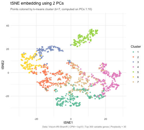
The animated figure disaplys how changing the number of principal components (PCs) that are used as an input to tSNE affects the resulting 2D embedding of Visium spatial transcriptomics spots. The animation transitions between tSNE embeddings computed from 2, 5, 10, 30, and 50 PCs. Each point represents a Visium spot that is colored by k-means clustering (k = 7, computed on PCs 1–10). When there are only 2 PCs, the clusters overlap heavily and there is very little biological variation. When the PC count is increased to 5, then to 10, clusters separated into very distinct groups. Moving beyond 10 PCs (30 and 50), the tSNE barely changes between frames. This means that the higher PC counts are most likely noise. This shows that only 5–10 PCs is enough to represent biological variation for tSNE, and any additional PCs result in diminishing returns.
The PC count is important because it is one of the first decisions for spatial transcriptomics analysis, meaning it impacts every downstream step (clustering, cell type identification, differential expression, biological conclusions). Having too few PCs runs the risks of merging cell types, masking biologically important ones. On the other hand, using too many PCs creates noise that can separate real clusters into sub-groups that prevent identification of true tissue structure.
Code
1
2
3
4
5
6
7
8
9
10
11
12
13
14
15
16
17
18
19
20
21
22
23
24
25
26
27
28
29
30
31
32
33
34
35
36
37
38
39
40
41
42
43
44
45
46
47
48
49
50
51
52
53
54
55
56
57
58
59
60
61
62
63
64
65
66
67
68
69
70
71
72
73
74
75
76
77
78
79
80
81
82
83
84
85
86
87
88
89
90
# Load data
setwd("/Users/emmameihofer/Documents/GitHub/genomic-data-visualization-2026")
data <- read.csv("data/Visium-IRI-ShamR_matrix.csv.gz")
pos <- data[, c('x', 'y')]
rownames(pos) <- data[, 1]
gexp <- data[, 4:ncol(data)]
rownames(gexp) <- data[, 1]

# Normalize:  CPM + log10
totgexp <- rowSums(gexp)
mat <- log10(gexp / totgexp * 1e6 + 1)

# Feature selection: top 300 variable genes
vg <- apply(mat, 2, var)
vargenes <- names(sort(vg, decreasing = TRUE)[1:300])
matsub <- mat[, vargenes]

# PCA
pcs <- prcomp(matsub, center = TRUE, scale. = FALSE)

# Run tSNE with varying numbers of PCs
library(Rtsne)

pc_counts <- c(2, 5, 10, 30, 50)
tsne_results <- lapply(pc_counts, function(k) {
  set.seed(42)  # same seed for fair comparison
  emb <- Rtsne(pcs$x[, 1:k], dims = 2, perplexity = 30)$Y
  colnames(emb) <- c('tSNE1', 'tSNE2')
  rownames(emb) <- rownames(matsub)
  emb
})
names(tsne_results) <- paste0(pc_counts, " PCs")

# K-means clustering (on PCs 1:10 as reference)
set.seed(42)
km <- kmeans(pcs$x[, 1:10], centers = 7)
cluster <- as.factor(km$cluster)

# Build combined data frame for animation
library(ggplot2)
library(gganimate)

df_list <- lapply(seq_along(pc_counts), function(i) {
  data.frame(
    cell = rownames(matsub),
    tSNE1 = tsne_results[[i]][, 1],
    tSNE2 = tsne_results[[i]][, 2],
    cluster = cluster,
    nPCs = paste0(pc_counts[i], " PCs")
  )
})
df_anim <- do.call(rbind, df_list)
df_anim$nPCs <- factor(df_anim$nPCs, levels = paste0(pc_counts, " PCs"))

# LLM Prompt:  How do I take my tSNE plots for each number of PCs and animate
# it with gganimate?
# Animated tSNE plot
anim <- ggplot(df_anim, aes(x = tSNE1, y = tSNE2, col = cluster, group = cell)) +
  geom_point(size = 1.5, alpha = 0.8) +
  scale_color_brewer(palette = "Set2") +
  transition_states(nPCs,
                    transition_length = 2,
                    state_length = 1) +
  labs(
    title = 'tSNE embedding using {closest_state}',
    subtitle = 'Points colored by k-means cluster (k=7, computed on PCs 1:10)',
    x = 'tSNE1',
    y = 'tSNE2',
    color = 'Cluster',
    caption = 'Data: Visium-IRI-ShamR | CPM + log10 | Top 300 variable genes | Perplexity = 30'
  ) +
  ease_aes('cubic-in-out') +
  theme_minimal() +
  theme(
    plot.title = element_text(face = "bold", size = 14),
    plot.subtitle = element_text(size = 10, color = "grey40"),
    plot.caption = element_text(size = 8, color = "grey50")
  )

#LLM Prompt:  Given this code, how do I save the GIF to my computer?
# Render
animate(anim, nframes = 150, fps = 15, width = 500, height = 450,
        renderer = gifski_renderer("hw3_varying_pcs_tsne.gif"))

# Store the rendered animation
rendered <- animate(anim, nframes = 150, fps = 15, width = 500, height = 450,
                    renderer = gifski_renderer())

# Now save it
anim_save("~/Downloads/hw3_varying_pcs_tsne.gif", animation = rendered)