Identification of TAL cells using Deconvolution

Compare your result with the clustering and differential expression analysis you did previously in HW3/4. Explain how your results are similar or different. Create a data visualization comparing all three analyses.
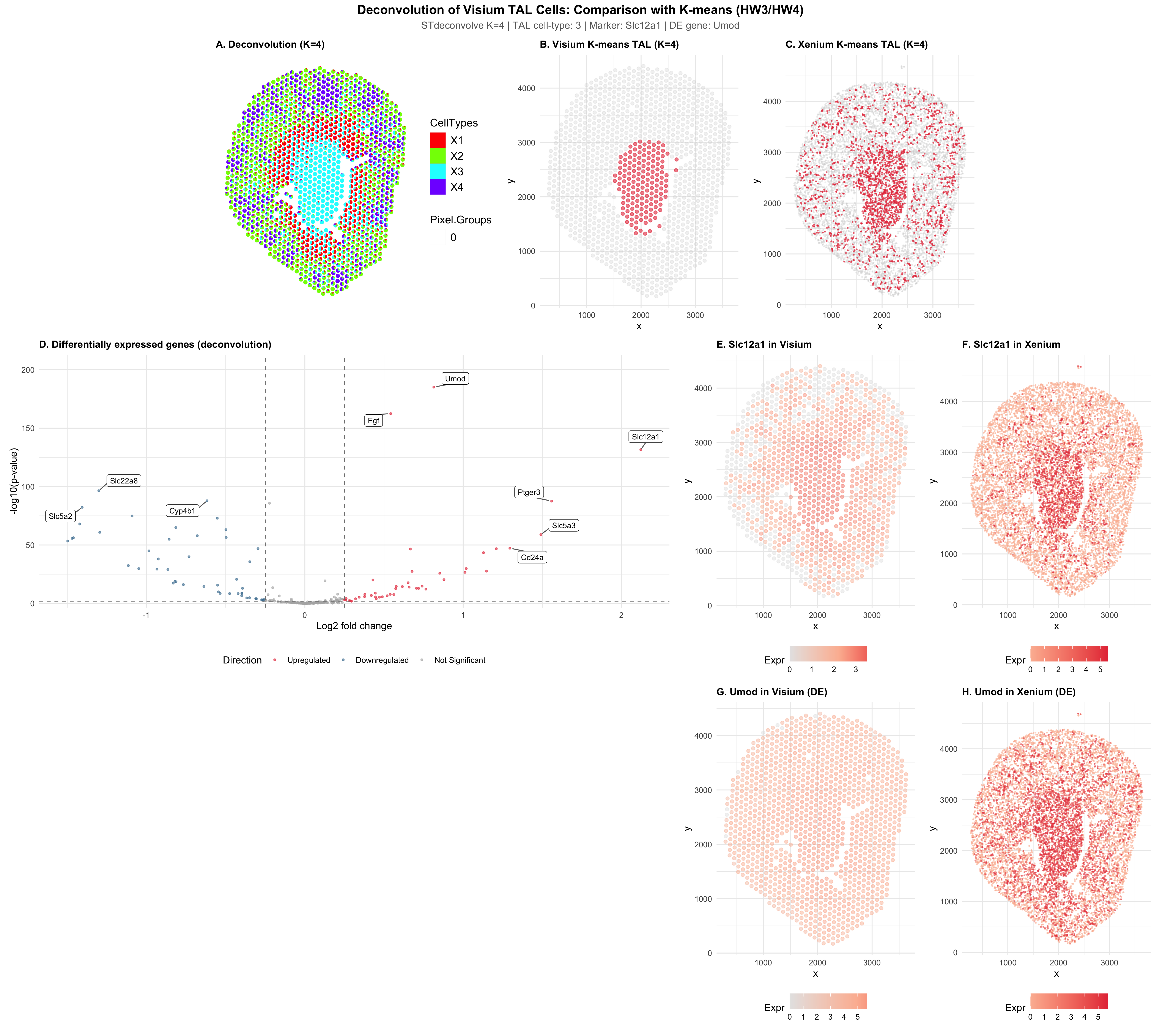
This visualization is a comparison of three approaches to identifying Thick Ascending Limb (TAL) cells in kidney tissue. It includes STdeconvolve deconvolution on Visium (this homework), K-means clustering on Visium (HW3), and K-means clustering on Xenium (HW4). All of the methods use K = 4, which was selected by STdeconvolve, so that there is a fair comparison. In HW3 I originally used k = 6 and in HW4 I used k = 8, but here it is standardized to K=4 for consistency.
In the first row of the visualization, spatial organization is compared for all three analysis methods. Panel A shows STdeconvolve results, which was visualized using vizAllTopics becuase scatterbar was not recognizing column names. Each Visium spot is a stacked bar showing the estimated proportions of K = 4 deconvolved cell-types. Unlike K-means, which assigns each spot a single identity, deconvolution shows when there is mixed cell-type composition within spots. Panels B and C show the TAL cluster in red, which was identified by K-means in both the Visium and Xenium datasets, with all other cells in grey. The TAL cells were localized to the medulla in all three analyses.
The second row shows the range of differential expression along with the specific TAL marker Slc12a1. Panel D is a volcano plot of genes differentially expressed between Visium spots with high vs low TAL proportion (from deconvolution). The known TAL markers (Slc12a1, Umod, Egf, Cd24a) were labeled. Panels E and F show Slc12a1 expression in both the Visium and Xenium tissues,reiterating the spatial patterns across different platforms.
The last row shows a differentially upregulated gene (Umod) that was identified from the deconvolution analysis. It was also visualized in both Visium (G) and Xenium (H), showing the DE finding at single-cell resolution.
All three approaches were able to identify TAL cells in the same anatomical region of the medulla. The same marker genes (Slc12a1, Umod, Egf) emerged as top upregulated genes, regardless of the method used. The main difference was that deconvolution was able to capture continuous variation in TAL proportion at each spot. This showed the existence of gradients at tissue boundaries that isn’t completely represented by K-means clustering.
Code
1
2
3
4
5
6
7
8
9
10
11
12
13
14
15
16
17
18
19
20
21
22
23
24
25
26
27
28
29
30
31
32
33
34
35
36
37
38
39
40
41
42
43
44
45
46
47
48
49
50
51
52
53
54
55
56
57
58
59
60
61
62
63
64
65
66
67
68
69
70
71
72
73
74
75
76
77
78
79
80
81
82
83
84
85
86
87
88
89
90
91
92
93
94
95
96
97
98
99
100
101
102
103
104
105
106
107
108
109
110
111
112
113
114
115
116
117
118
119
120
121
122
123
124
125
126
127
128
129
130
131
132
133
134
135
136
137
138
139
140
141
142
143
144
145
146
147
148
149
150
151
152
153
154
155
156
157
158
159
160
161
162
163
164
165
166
167
168
169
170
171
172
173
174
175
176
177
178
179
180
181
182
183
184
185
186
187
188
189
190
191
192
193
194
195
196
197
198
199
200
201
202
203
204
205
206
207
208
209
210
211
212
213
214
215
216
217
218
219
220
221
222
223
224
225
226
227
228
229
230
231
232
233
234
235
236
237
238
239
240
241
242
243
244
245
246
247
248
249
250
251
252
253
254
255
256
257
258
259
260
261
262
263
264
265
266
267
268
269
270
library(ggplot2)
library(patchwork)

## read in Visium data
setwd("/Users/emmameihofer/Documents/GitHub/genomic-data-visualization-2026")
data <- read.csv("data/Visium-IRI-ShamR_matrix.csv.gz")
pos <- data[,c('x', 'y')]
rownames(pos) <- data[,1]
gexp <- data[, 4:ncol(data)]
rownames(gexp) <- data[,1]
dim(gexp)

# read in Xenium data
xdata <- read.csv("data/Xenium-IRI-ShamR_matrix.csv.gz")
set.seed(42)
xdata <- xdata[sample(1:nrow(xdata), 10000),]
xpos <- xdata[,c('x', 'y')]
rownames(xpos) <- xdata[,1]
xgexp <- xdata[, 4:ncol(xdata)]
rownames(xgexp) <- xdata[,1]

# Shared genes
genes.have <- intersect(colnames(xgexp), colnames(gexp))

# STdeconvolve ON VISIUM
library(STdeconvolve)

gexp.sub <- gexp[, genes.have]
ldas <- fitLDA(gexp.sub, Ks = c(3, 4, 5, 6, 7))
optLDA <- optimalModel(models = ldas, opt = "kneed")
results <- getBetaTheta(optLDA, perc.filt = 0.05, betaScale = 1000)

deconProp <- results$theta
deconGexp <- results$beta
K <- ncol(deconProp)

# Print top genes per cell-type
for (i in 1:K) {
  cat("Cell-type", i, ":", names(head(sort(deconGexp[i,], decreasing = TRUE), 5)), "\n")
}

# Identify TAL cell-type (highest Slc12a1 loading)
ct_scores <- deconGexp[, 'Slc12a1']
ct <- names(which.max(ct_scores))
cat("TAL cell-type:", ct, "\n")

# VISIUM K-MEANS (same K as deconvolution for comparison)
totgexp <- rowSums(gexp)
mat <- log10(gexp / totgexp * 1e6 + 1)
vg <- apply(mat, 2, var)
vargenes <- names(sort(vg, decreasing = TRUE)[1:500])
matsub <- mat[, vargenes]

pcs <- prcomp(matsub, center = TRUE, scale. = FALSE)

set.seed(42)
km_vis <- kmeans(pcs$x[, 1:15], centers = K)
vis_clusters <- as.factor(km_vis$cluster)

# Find Visium cluster most enriched for Slc12a1
vis_cl_means <- tapply(mat[, 'Slc12a1'], vis_clusters, mean)
vis_cl_interest <- names(which.max(vis_cl_means))
cat("Visium TAL cluster:", vis_cl_interest, "\n")

# XENIUM K-MEANS (same K as deconvolution for comparison)
xtotgexp <- rowSums(xgexp)
xmat <- log10(xgexp / xtotgexp * 1e6 + 1)
xpcs <- prcomp(xmat, center = TRUE, scale. = FALSE)

set.seed(42)
km_xen <- kmeans(xpcs$x[, 1:15], centers = K, nstart = 10)
xen_clusters <- as.factor(km_xen$cluster)

# Find Xenium cluster most enriched for Slc12a1
xen_cl_means <- tapply(xmat[, 'Slc12a1'], xen_clusters, mean)
xen_cl_interest <- names(which.max(xen_cl_means))
cat("Xenium TAL cluster:", xen_cl_interest, "\n")

# DIFFERENTIAL EXPRESSION (deconvolution-based on Visium)
mat_sub_norm <- log10(gexp.sub / rowSums(gexp.sub) * 1e6 + 1)

ct_prop <- deconProp[, ct]
high_spots <- names(ct_prop[ct_prop > median(ct_prop)])
low_spots <- names(ct_prop[ct_prop <= median(ct_prop)])

# Two-sided test
de_pvals_up <- sapply(colnames(mat_sub_norm), function(g) {
  wilcox.test(mat_sub_norm[high_spots, g], mat_sub_norm[low_spots, g],
              alternative = 'greater')$p.value
})
de_pvals_down <- sapply(colnames(mat_sub_norm), function(g) {
  wilcox.test(mat_sub_norm[high_spots, g], mat_sub_norm[low_spots, g],
              alternative = 'less')$p.value
})
de_pvals_twosided <- sapply(colnames(mat_sub_norm), function(g) {
  wilcox.test(mat_sub_norm[high_spots, g], mat_sub_norm[low_spots, g],
              alternative = 'two.sided')$p.value
})

mean_high <- colMeans(mat_sub_norm[high_spots, ])
mean_low <- colMeans(mat_sub_norm[low_spots, ])
log2fc <- mean_high - mean_low

de_results <- data.frame(
  gene = names(de_pvals_twosided),
  pval = de_pvals_twosided,
  pval_up = de_pvals_up,
  pval_down = de_pvals_down,
  log2fc = log2fc,
  neglog10p = -log10(de_pvals_twosided)
)

# Cap Inf values (from p-values of exactly 0)
max_finite <- max(de_results$neglog10p[is.finite(de_results$neglog10p)])
de_results$neglog10p[is.infinite(de_results$neglog10p)] <- max_finite * 1.05

de_results <- de_results[order(de_results$pval), ]

cat("\nTop 15 DE genes (deconvolution-based):\n")
print(head(de_results[order(de_results$pval_up), ], 15))

# Pick DE gene: top significant upregulated gene that isn't Slc12a1
de_up_sorted <- de_results[order(de_results$pval_up), ]
de_up_sig <- de_up_sorted[de_up_sorted$pval_up < 0.05 & de_up_sorted$log2fc > 0, ]
de_gene <- de_up_sig$gene[de_up_sig$gene != 'Slc12a1'][1]
cat("DE gene for visualization:", de_gene, "\n")

# BUILD FIGURE
library(ggplot2)
library(patchwork)
library(ggrepel)

theme_hw <- theme_minimal(base_size = 11) +
  theme(plot.title = element_text(face = "bold", size = 11),
        legend.position = "bottom",
        plot.margin = margin(5, 10, 5, 5))

# Used vizAllTopics because scatterbar had a functional error
# Panel A: STdeconvolve proportions via vizAllTopics
pos_decon <- data.frame(x = pos[rownames(deconProp), 'x'],
                        y = pos[rownames(deconProp), 'y'])
rownames(pos_decon) <- rownames(deconProp)
pA <- vizAllTopics(deconProp, pos_decon, r = 40) +
  labs(title = paste0("A. Deconvolution (K=", K, ")")) +
  theme(plot.title = element_text(face = "bold", size = 11))

# Panel B: Visium K-means TAL cluster on tissue
df_vis <- data.frame(pos, cluster = vis_clusters)
df_vis_other <- df_vis[df_vis$cluster != vis_cl_interest, ]
df_vis_coi <- df_vis[df_vis$cluster == vis_cl_interest, ]

pB <- ggplot() +
  geom_point(data = df_vis_other, aes(x = x, y = y),
             color = "#D3D3D3", size = 1.5, alpha = 0.3) +
  geom_point(data = df_vis_coi, aes(x = x, y = y),
             color = "#E63946", size = 1.5, alpha = 0.6) +
  coord_fixed() +
  labs(title = paste0("B. Visium K-means TAL (K=", K, ")")) +
  theme_hw + theme(legend.position = "none")

# Panel C: Xenium K-means TAL cluster on tissue
df_xen <- data.frame(xpos, cluster = xen_clusters)
df_xen_other <- df_xen[df_xen$cluster != xen_cl_interest, ]
df_xen_coi <- df_xen[df_xen$cluster == xen_cl_interest, ]

pC <- ggplot() +
  geom_point(data = df_xen_other, aes(x = x, y = y),
             color = "#D3D3D3", size = 0.3, alpha = 0.3) +
  geom_point(data = df_xen_coi, aes(x = x, y = y),
             color = "#E63946", size = 0.3, alpha = 0.6) +
  coord_fixed() +
  labs(title = paste0("C. Xenium K-means TAL (K=", K, ")")) +
  theme_hw + theme(legend.position = "none")

# LLM Prompt:  How do I plot the bidirectional volcano plot like the one
# I used in this figure (hw4) using the deconvolution visium data?
# Panel D: Bidirectional volcano plot
de_results$direction <- ifelse(de_results$pval < 0.05 & de_results$log2fc > 0.25, "Upregulated",
                        ifelse(de_results$pval < 0.05 & de_results$log2fc < -0.25, "Downregulated",
                        "Not Significant"))
de_results$direction <- factor(de_results$direction,
                               levels = c("Upregulated", "Downregulated", "Not Significant"))

top5_up <- head(de_results$gene[de_results$direction == "Upregulated"], 5)
top3_down <- head(de_results$gene[de_results$direction == "Downregulated"], 3)
tal_markers <- c('Slc12a1', 'Umod', 'Egf', 'Cd24a')
available_markers <- tal_markers[tal_markers %in% de_results$gene]
label_genes <- unique(c(top5_up, top3_down, available_markers, de_gene))
de_results$label <- ifelse(de_results$gene %in% label_genes, de_results$gene, "")

volcano_cols <- c("Upregulated" = "#E63946", "Downregulated" = "#457B9D",
                  "Not Significant" = "grey70")

pD <- ggplot(de_results, aes(x = log2fc, y = neglog10p)) +
  geom_point(aes(col = direction), size = 0.8, alpha = 0.6) +
  scale_color_manual(values = volcano_cols) +
  geom_label_repel(aes(label = label), size = 3, max.overlaps = 20,
                   box.padding = 0.5, point.padding = 0.3,
                   min.segment.length = 0, segment.color = "grey40",
                   fill = "white", label.size = 0.2) +
  geom_hline(yintercept = -log10(0.05), linetype = "dashed", color = "grey50") +
  geom_vline(xintercept = c(-0.25, 0.25), linetype = "dashed", color = "grey50") +
  scale_y_continuous(expand = expansion(mult = c(0.02, 0.15))) +
  labs(title = "D. Differentially expressed genes (deconvolution)",
       x = "Log2 fold change", y = "-log10(p-value)", color = "Direction") +
  theme_hw

# Panel E: Slc12a1 in Visium tissue
df_vis_gene <- data.frame(pos, gene = mat[, 'Slc12a1'])
df_vis_gene <- df_vis_gene[order(df_vis_gene$gene), ]
pE <- ggplot(df_vis_gene, aes(x = x, y = y, col = gene)) +
  geom_point(size = 1.5, alpha = 0.5) +
  scale_color_gradient2(low = "grey90", mid = "#FCBBA1", high = "#E63946",
                        midpoint = median(df_vis_gene$gene)) +
  coord_fixed() +
  labs(title = "E. Slc12a1 in Visium", color = "Expr") +
  theme_hw

# Panel F: Slc12a1 in Xenium tissue
df_xen_gene <- data.frame(xpos, gene = xmat[, 'Slc12a1'])
df_xen_gene <- df_xen_gene[order(df_xen_gene$gene), ]
pF <- ggplot(df_xen_gene, aes(x = x, y = y, col = gene)) +
  geom_point(size = 0.3, alpha = 0.5) +
  scale_color_gradient2(low = "grey90", mid = "#FCBBA1", high = "#E63946",
                        midpoint = median(df_xen_gene$gene)) +
  coord_fixed() +
  labs(title = "F. Slc12a1 in Xenium", color = "Expr") +
  theme_hw

# Panel G: DE gene in Visium tissue
df_vis_de <- data.frame(pos, gene = mat_sub_norm[, de_gene])
df_vis_de <- df_vis_de[order(df_vis_de$gene), ]
pG <- ggplot(df_vis_de, aes(x = x, y = y, col = gene)) +
  geom_point(size = 1.5, alpha = 0.5) +
  scale_color_gradient2(low = "grey90", mid = "#FCBBA1", high = "#E63946",
                        midpoint = median(df_vis_de$gene)) +
  coord_fixed() +
  labs(title = paste0("G. ", de_gene, " in Visium (DE)"), color = "Expr") +
  theme_hw

# Panel H: DE gene in Xenium tissue
df_xen_de <- data.frame(xpos, gene = xmat[, de_gene])
df_xen_de <- df_xen_de[order(df_xen_de$gene), ]
pH <- ggplot(df_xen_de, aes(x = x, y = y, col = gene)) +
  geom_point(size = 0.3, alpha = 0.5) +
  scale_color_gradient2(low = "grey90", mid = "#FCBBA1", high = "#E63946",
                        midpoint = median(df_xen_de$gene)) +
  coord_fixed() +
  labs(title = paste0("H. ", de_gene, " in Xenium (DE)"), color = "Expr") +
  theme_hw

# ASSEMBLE AND SAVE
top_row <- pA + pB + pC + plot_layout(nrow = 1)
mid_row <- pD + pE + pF + plot_layout(nrow = 1)
bot_row <- plot_spacer() + pG + pH + plot_layout(nrow = 1)

final <- (top_row / mid_row / bot_row) +
  plot_annotation(
    title = 'Deconvolution of Visium TAL Cells: Comparison with K-means (HW3/HW4)',
    subtitle = paste0('STdeconvolve K=', K, ' | TAL cell-type: ', ct,
                      ' | Marker: Slc12a1 | DE gene: ', de_gene),
    theme = theme(
      plot.title = element_text(face = "bold", size = 14, hjust = 0.5),
      plot.subtitle = element_text(size = 11, hjust = 0.5, color = "grey40")
    )
  )

ggsave("~/Downloads/emeihof1_HW5.png", final,
       width = 18, height = 16, dpi = 300, bg = "white")
cat("\n=== Saved to ~/Downloads/emeihof1_HWEC2.png ===\n")