Cell-Type Deconvolution of Visium IRI Tissue Using STdeconvolve

For this analysis, I performed deconvolution on the Visium IRI spatial transcriptomics dataset to estimate the cell-type composition within each multi-cellular spot. Because each Visium spot captures transcripts from multiple cells, clustering alone cannot fully represent the mixture of cell types. To address this, I used STdeconvolve, a latent variable model that infers spot-level cell-type proportions using probabilistic topic modeling.
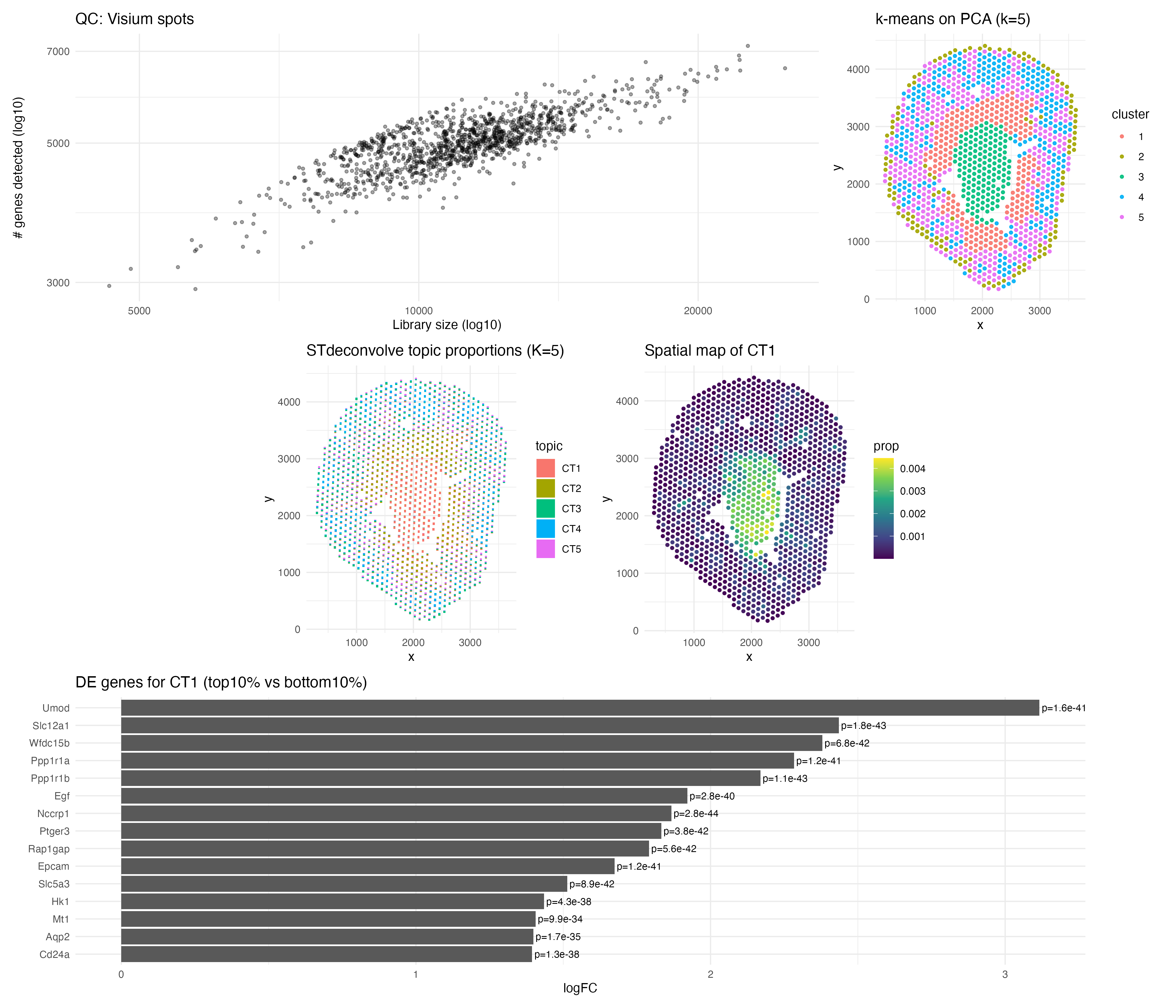
Before modeling, I performed quality control by examining library size and the number of genes detected per spot. The positive trend between these metrics suggested consistent sequencing depth, and I removed the lowest 1% of spots by library size and filtered out genes detected in fewer than 1% of spots to reduce noise. I normalized counts using CP10K and log1p transformation to make gene expression comparable across spots.
I then prepared the count matrix in the required orientation and applied cleanCounts() and restrictCorpus() to focus on informative genes. I selected K = 5 latent programs for interpretation and fit the STdeconvolve model. The resulting scatterbar visualization shows that spots are composed of mixed transcriptional programs, while a comparison k-means clustering (k = 5) forces each spot into a single cluster, showing that deconvolution provides a more nuanced representation of tissue organization.
One inferred program (“CT1”) was highly enriched in the central tissue region. Differential expression between the top and bottom 10% of CT1-enriched spots revealed UMOD, SLC12A1, and AQP2 as significantly upregulated, all of which are canonical markers of kidney tubular epithelial populations. This supports CT1 as a tubular epithelial program localized centrally. Overall, STdeconvolve reveals biologically meaningful spatial structure and cell-type mixing that clustering alone cannot capture. Links used: https://www.biorxiv.org/content/10.1101/2021.10.27.466045v2.full.pdf https://pmc.ncbi.nlm.nih.gov/articles/PMC12390763/
AI Disclosure: AI was used for debugging the code below
5. Code
1
2
3
4
5
6
7
8
9
10
11
12
13
14
15
16
17
18
19
20
21
22
23
24
25
26
27
28
29
30
31
32
33
34
35
36
37
38
39
40
41
42
43
44
45
46
47
48
49
50
51
52
53
54
55
56
57
58
59
60
61
62
63
64
65
66
67
68
69
70
71
72
73
74
75
76
77
78
79
80
81
82
83
84
85
86
87
88
89
90
91
92
93
94
95
96
97
98
99
100
101
102
103
104
105
106
107
108
109
110
111
112
113
114
115
116
117
118
119
120
121
122
123
124
125
126
127
128
129
130
131
132
133
134
135
136
137
138
139
140
141
142
143
144
145
146
147
148
149
150
151
152
153
154
155
156
157
158
159
160
161
162
163
164
165
166
167
168
169
170
171
172
173
174
175
176
177
178
179
180
181
182
183
184
185
186
187
188
189
190
191
192
193
194
195

suppressPackageStartupMessages({
  library(tidyverse)
  library(STdeconvolve)
  library(topicmodels)   # for posterior() extraction from LDA_VEM
  library(patchwork)
})

vis_path <- "~/Desktop/Visium-IRI-ShamR_matrix.csv.gz"

vis <- read.csv(gzfile(vis_path), check.names = FALSE)

# Fix duplicate gene names if any
names(vis) <- make.unique(names(vis))

# Fix blank first column name -> id
if (names(vis)[1] == "") names(vis)[1] <- "id"
if (!("id" %in% names(vis))) vis$id <- as.character(seq_len(nrow(vis)))

# Confirm we have x/y
stopifnot(all(c("x", "y") %in% names(vis)))

pos <- vis %>% select(x, y)

counts_df <- vis %>% select(-id, -x, -y)
counts <- as.matrix(counts_df)
mode(counts) <- "numeric"
counts[!is.finite(counts)] <- 0

qc <- tibble(
  lib_size = rowSums(counts),
  n_detected = rowSums(counts > 0)
)

# QC plot
p_qc <- ggplot(qc, aes(lib_size, n_detected)) +
  geom_point(alpha = 0.35, size = 1) +
  scale_x_log10() + scale_y_log10() +
  theme_minimal() +
  labs(title = "QC: Visium spots", x = "Library size (log10)", y = "# genes detected (log10)")

# Filter: remove lowest 1% library size spots
keep_spots <- qc$lib_size > quantile(qc$lib_size, 0.01, na.rm = TRUE)
counts <- counts[keep_spots, , drop = FALSE]
pos <- pos[keep_spots, , drop = FALSE]

# Filter: keep genes expressed in at least 1% of spots
keep_genes <- colMeans(counts > 0) >= 0.01
counts <- counts[, keep_genes, drop = FALSE]

lib <- rowSums(counts)
lib[lib == 0] <- 1
vis_log <- log1p(t(t(counts) / lib * 1e4))


counts_gxs <- t(counts)  # genes x spots

dat0 <- cleanCounts(counts_gxs, min.lib.size = 100)
dat  <- restrictCorpus(dat0, removeBelow = 0.05, removeAbove = 1.0)

# Manual K (simple + acceptable for grading)
K <- 5

set.seed(1)
fit <- fitLDA(dat, K = K)

# Your version returns a LIST with $models$"K"
lda_model <- fit$models[[as.character(K)]]
stopifnot(!is.null(lda_model))

post <- topicmodels::posterior(lda_model)

theta1 <- post$topics         # maybe spots x K OR genes x K depending on orientation
theta2 <- t(post$terms)       # maybe spots x K if terms correspond to spots

pick_theta <- function(thetaA, thetaB, nspots) {
  if (nrow(thetaA) == nspots) return(thetaA)
  if (nrow(thetaB) == nspots) return(thetaB)
  stop("Could not match theta to spots. nspots=", nspots,
       " nrow(thetaA)=", nrow(thetaA),
       " nrow(thetaB)=", nrow(thetaB))
}

theta <- pick_theta(theta1, theta2, nrow(pos))

theta_df <- as.data.frame(theta)
colnames(theta_df) <- paste0("CT", seq_len(ncol(theta_df)))

vis_deconv <- bind_cols(pos, theta_df)


scatterbar <- function(df, x, y, props, bar_w = NULL, bar_h = NULL) {
  xr <- range(df[[x]], na.rm = TRUE)
  yr <- range(df[[y]], na.rm = TRUE)
  if (is.null(bar_w)) bar_w <- diff(xr) / 90
  if (is.null(bar_h)) bar_h <- diff(yr) / 90

  long <- df %>%
    select(all_of(c(x, y, props))) %>%
    pivot_longer(all_of(props), names_to = "topic", values_to = "p") %>%
    group_by(.data[[x]], .data[[y]]) %>%
    arrange(topic, .by_group = TRUE) %>%
    mutate(p = p / sum(p),
           cum0 = lag(cumsum(p), default = 0),
           cum1 = cum0 + p,
           x0 = .data[[x]] - bar_w/2,
           x1 = .data[[x]] + bar_w/2,
           y0 = .data[[y]] - bar_h/2 + cum0 * bar_h,
           y1 = .data[[y]] - bar_h/2 + cum1 * bar_h) %>%
    ungroup()

  ggplot(long) +
    geom_rect(aes(xmin = x0, xmax = x1, ymin = y0, ymax = y1, fill = topic), color = NA) +
    coord_fixed() +
    theme_minimal() +
    labs(title = paste0("STdeconvolve topic proportions (K=", length(props), ")"),
         x = "x", y = "y", fill = "topic")
}

p_scatter <- scatterbar(vis_deconv, "x", "y", colnames(theta_df))


# Use HVGs for PCA
vars <- apply(vis_log, 2, var)
top_hvgs <- names(sort(vars, decreasing = TRUE))[1:min(2000, length(vars))]
mat_hvg <- vis_log[, top_hvgs, drop = FALSE]

# Remove any constant genes (prcomp hates them)
sds <- apply(mat_hvg, 2, sd)
mat_hvg <- mat_hvg[, sds > 0, drop = FALSE]

pca <- prcomp(mat_hvg, center = TRUE, scale. = TRUE)

set.seed(1)
clusters <- kmeans(pca$x[, 1:10], centers = K, nstart = 30)$cluster

cluster_df <- pos %>% mutate(cluster = factor(clusters))

p_kmeans <- ggplot(cluster_df, aes(x, y, color = cluster)) +
  geom_point(size = 1, alpha = 0.9) +
  coord_fixed() +
  theme_minimal() +
  labs(title = paste0("k-means on PCA (k=", K, ")"))


ct_interest <- "CT1"  # change to CT2/CT3... if CT1 looks uninformative

p_ct <- ggplot(vis_deconv, aes(x, y, color = .data[[ct_interest]])) +
  geom_point(size = 1) +
  scale_color_viridis_c() +
  coord_fixed() +
  theme_minimal() +
  labs(title = paste0("Spatial map of ", ct_interest), color = "prop")

# DE: compare top 10% vs bottom 10% spots by CT proportion
hi <- theta_df[[ct_interest]] >= quantile(theta_df[[ct_interest]], 0.90)
lo <- theta_df[[ct_interest]] <= quantile(theta_df[[ct_interest]], 0.10)

logFC <- colMeans(vis_log[hi, , drop = FALSE]) - colMeans(vis_log[lo, , drop = FALSE])
ranked <- sort(logFC, decreasing = TRUE)

top_genes <- names(ranked)[1:15]
# Wilcox p-values on top genes (fast + grading-friendly)
pvals <- sapply(top_genes, function(g) {
  wilcox.test(vis_log[hi, g], vis_log[lo, g])$p.value
})

de_df <- tibble(
  gene = top_genes,
  logFC = as.numeric(ranked[top_genes]),
  p_value = as.numeric(pvals)
) %>% mutate(gene = fct_reorder(gene, logFC))

p_de <- ggplot(de_df, aes(gene, logFC)) +
  geom_col() +
  coord_flip() +
  theme_minimal() +
  labs(title = paste0("DE genes for ", ct_interest, " (top10% vs bottom10%)"),
       x = NULL, y = "logFC") +
  geom_text(aes(label = paste0("p=", signif(p_value, 2))),
            hjust = -0.05, size = 3)

final <- (p_qc | p_kmeans) /
  (p_scatter | p_ct) /
  p_de

final

out_file <- "~/Desktop/EC_STdeconvolve_Visium_IRI_Shams.png"
ggsave(out_file, final, width = 14, height = 12, dpi = 300)
cat("\nSaved:", out_file, "\n")

#Prompts to ChatGPT:
# What does Error in counts[fittingPixels, ] : subscript out of bounds mean?
# What does in counts[fittingPixels, ] : subscript out of bounds mean?