A deconvolution approach to identify Proximal Convoluted Tubule segments

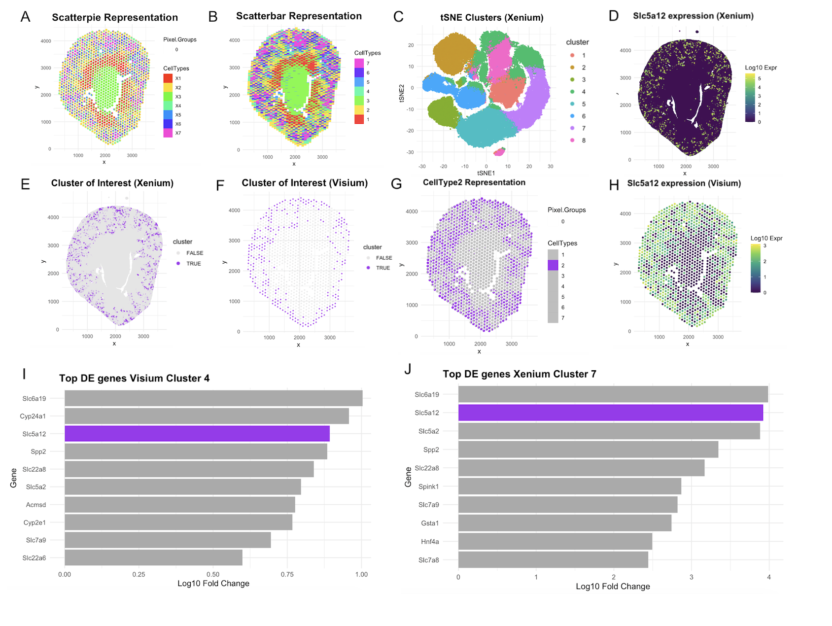
This visualization assesses a coronal kidney tissue section using deconvolution and clustering across Xenium and Visium Platforms. Using STdeconvolve, Panel A depicts 7 distinct cell types in a scatterpie visualization. Each spot is able to show the proportion of each cell type within it. Panel B uses the scatterbar format created by our guest lecturer Dee. Each proportion within each spot is encoded with position instead of angle with the form of stacked bars. Panel C is a callback to tSNE clustering done in HW, helping us identify spatially that our cluster of interest investigated in that HW was cluster 7 in this iteration of tSNE run (same seed was chosen, but cluster numbering and coloring was different). Panel E visualizes this cluster of interest in physical space. Panel F finds that in Visium data, cluster 4 was most analogous to the Xenium’s cluster 7 spatially. This was verified by differentially gene analysis in Panels I and J, where these respective clusters also displayed Slc5a12 as a top 3 differentially upregulated gene. Panel G was able to isolate Celltype 2 as analogous to these clusters and showed a much clearer pattern of tubule arrangement than the disjointed visium spots in panel F. This confirmed our previous hypothesis from HW 4, that since spots are 55um, PCTs are present in spots with other distinct cell-types that may get labelled in a different cluster. With deconvolution, we were able to create resolution to a greater extent than just Visium alone. The pattern was closer to Xenium’s displaying the move towards higher cellular resolution. Panels D and H display gene expression of Slc5a12, a marker for PCT segments to further spatially map to the cluster and cell types.
Code
1
2
3
4
5
6
7
8
9
10
11
12
13
14
15
16
17
18
19
20
21
22
23
24
25
26
27
28
29
30
31
32
33
34
35
36
37
38
39
40
41
42
43
44
45
46
47
48
49
50
51
52
53
54
55
56
57
58
59
60
61
62
63
64
65
66
67
68
69
70
71
72
73
74
75
76
77
78
79
80
81
82
83
84
85
86
87
88
89
90
91
92
93
94
95
96
97
98
99
100
101
102
103
104
105
106
107
108
109
110
111
112
113
114
115
116
117
118
119
120
121
122
123
124
125
126
127
128
129
130
131
132
133
134
135
136
137
138
139
140
141
142
143
144
145
146
147
148
149
150
151
152
153
154
155
156
157
158
159
160
161
162
163
164
165
166
167
168
169
170
171
172
173
174
175
176
177
178
179
180
181
182
183
184
185
186
187
188
189
190
191
192
193
194
195
196
197
198
199
200
201
202
203
204
205
206
207
208
209
210
211
212
213
214
215
216
217
218
219
220
221
222
223
224
225
226
227
228
229
230
231
232
233
234
235
236
237
238
239
240
241
242
243
244
245
246
247
248
library(STdeconvolve)
library(ggplot2)
library(patchwork)
library(Rtsne)
library(scatterpie)
library(scatterbar)

data <- read.csv('~/Desktop/GDV/Visium-IRI-ShamR_matrix.csv.gz')
pos <- data[,c('x', 'y')]
rownames(pos) <- data[,1]
gexp <- data[, 4:ncol(data)]
rownames(gexp) <- data[,1]
head(pos)
gexp[1:5,1:5]
dim(gexp)
totgexp <- rowSums(gexp)

genes <- read.csv('~/Desktop/GDV/Xenium-IRI-ShamR_matrix.csv.gz')
genes <- colnames(genes)[4:ncol(genes)]
genes.have <- intersect(genes, colnames(gexp))
length(genes.have)

# subset Visium to just Xenium genes
gexp.sub <- gexp[, genes.have]
range(rowSums(gexp.sub))
mat <- log10(gexp.sub/totgexp * 1e6 + 1)
# apply deconvolution to Visium data
# compare with Xenium data
# deconvolution
ldas <- fitLDA(gexp.sub, Ks = c(3,4,5,6,7))
optLDA <- optimalModel(models = ldas, opt = "7")
results <- getBetaTheta(optLDA, perc.filt = 0.05, betaScale = 1000)
# theta is cell-type proportions
# beta is cell-type-specific gene expression
head(results$theta)
head(results$beta)
head(sort(results$beta[1,], decreasing=TRUE))

deconProp <- results$theta
deconGexp <- results$beta
g1 <- vizAllTopics(deconProp, pos, r = 40)+
  labs(title = "Scatterpie Representation", x="x", y="y")+
  coord_fixed() +
  theme_minimal()+
  theme(plot.title = element_text(size = 9, face = "bold"))
g1

g1_sp <- vizAllTopics(deconProp, pos, r = 40)+
  labs(title = "CellType2 Representation", x="x", y="y")+
  coord_fixed() +
  scale_fill_manual(
    values = c(
      "X1" = "gray", "X2" = "purple", "X3" = "gray",
      "X4" = "gray", "X5" = "gray", "X6" = "gray",
      "X7" = "gray"
    ), labels = function(x) gsub("^X", "", x)
  ) +
  theme_minimal()+
  theme(plot.title = element_text(size = 9, face = "bold"))
g1_sp

g2_scatterbar <- scatterbar(data = as.data.frame(deconProp), xy = pos, padding_x = 0.2, padding_y = 0.2, legend_title = "CellTypes") +
  labs(title = "Scatterbar Representation", y="y") +
  theme_minimal() +
  coord_fixed()+
  theme(plot.title = element_text(size = 10, face = "bold"))
g2_scatterbar
pcs <- prcomp(gexp.sub)
df <- data.frame(pcs$x[,1:2], deconProp)
emb <- Rtsne::Rtsne(gexp.sub)$Y
colnames(emb) <- c('tSNE1', 'tSNE2')
df <- data.frame(emb, deconProp)
head(df)

head(sort(deconGexp[3,], decreasing=TRUE))
g <- 'Slc5a12'
deconGexp[, g]
df <- data.frame(emb, pos, gene=log10(gexp.sub[rownames(pos),g]+1))
g3 <- ggplot(df, aes(x=x, y=y, col=gene)) +
  geom_point() +
  coord_fixed() +
  scale_color_viridis_c(name="Log10 Expr")+
  labs(title = paste("Slc5a12 expression with Deconvolution")) +
  theme(plot.title = element_text(size = 9, face = "bold", hjust=0.5))+
  theme_minimal()
g3

pcs <- prcomp(mat, center = TRUE, scale = FALSE)
plot(pcs$sdev[1:50]) #first 10 pcs chosen based on this plot
set.seed(42)
tsne <- Rtsne::Rtsne(pcs$x[, 1:10], dims=2, perplexity=30, verbose=TRUE) #verbose parameter added for troubleshooting
emb <- tsne$Y
rownames(emb) <- rownames(mat)
colnames(emb) <- c('tSNE1', 'tSNE2')
head(emb)

clusters <- as.factor(kmeans(pcs$x[,1:10], centers = 6)$cluster)
df_clusters <- data.frame(pos, pcs$x[,1:10], emb, cluster = clusters)
df_clusters$gene_expr <- mat[, "Slc5a12"]
pvis_s <- ggplot(df_clusters, aes(x=x, y=y, color=gene_expr)) +
  geom_point(size=1) +
  coord_fixed() +
  scale_color_viridis_c(name = "Log10 Expr") +
  theme_minimal() +
  labs(title = paste(target_gene, "expression (Visium)")) +
  theme(plot.title = element_text(size = 9, face = "bold"))
pvis_s

pvis_c <- ggplot(df_clusters, aes(x=x, y=y, color=cluster)) +
  geom_point(size = 0.8, alpha=0.8) +
  coord_fixed() +
  theme_minimal() +
  labs(title = "Clusters in physical space") +
  theme(plot.title = element_text(size = 9, face = "bold"))
pvis_c

pvis_t <- ggplot(df_clusters, aes(x=tSNE1, y=tSNE2, color=cluster)) +
  geom_point(size = 0.8, alpha=0.8) +
  coord_fixed() +
  theme_minimal() +
  labs(title = "tSNE Clusters (Visium)") +
  theme(plot.title = element_text(size = 9, face = "bold"))
pvis_t

target_cluster <- 4
#target cluster in physical space
pvis_coi <- ggplot(df_clusters, aes(x=x, y=y, color=cluster == target_cluster)) +
  geom_point(size=0.5, alpha = 0.7) +
  coord_fixed() +
  scale_color_manual(values=c("grey90", "purple")) +
  theme_minimal() +
  labs(title="Cluster of Interest (Visium)") +
  guides(color = guide_legend(override.aes = list(size = 2, alpha = 1))) +
  theme(plot.title = element_text(size = 9, face = "bold"))
pvis_coi

cluster_dx <- which(clusters == 4)
other_dx <- which(clusters != 4)
#mean expression
mean_in <- colMeans(mat[cluster_dx, ])
mean_out <- colMeans(mat[other_dx, ])
logFC <- mean_in - mean_out #log fold change
#top 10 genes upregulated in Cluster 3
top_genes <- sort(logFC, decreasing = TRUE)[1:10]
print(top_genes)
dx_df <- data.frame(gene = names(top_genes), logFC = as.numeric(top_genes))
dx_df$color_group <- ifelse(dx_df$gene == "Slc5a12", "highlight", "other")
p_vis_de <- ggplot(dx_df, aes(x = reorder(gene, logFC), y = logFC, fill = color_group)) +
  geom_bar(stat = "identity") +
  scale_fill_manual(values = c("highlight" = "purple", "other" = "darkgray")) +
  coord_flip() +
  theme_minimal() +
  theme(legend.position = "none") +
  labs(title = "Top DE genes Visium Cluster 4", x = "Gene", y = "Log10 Fold Change")+
  theme(plot.title = element_text(size = 9, face = "bold"))
p_vis_de
#### xenium
data <- read.csv('~/Desktop/GDV/Xenium-IRI-ShamR_matrix.csv.gz')
pos <- data[,c('x', 'y')]
rownames(pos) <- data[,1]
gexp <- data[, 4:ncol(data)]
rownames(gexp) <- data[,1]
head(pos)
gexp[1:5,1:5]
dim(gexp)
totgexp <- rowSums(gexp)
#normalizing the data
mat <- log10(gexp/totgexp * 1e6 + 1)
pcs <- prcomp(mat, center = TRUE, scale = FALSE)
plot(pcs$sdev[1:50]) #first 10 pcs chosen based on this plot
set.seed(42)

###Xenium analysis
tsne <- Rtsne::Rtsne(pcs$x[, 1:10], dims=2, perplexity=30, verbose=TRUE) #verbose parameter added for troubleshooting
emb <- tsne$Y
rownames(emb) <- rownames(mat)
colnames(emb) <- c('tSNE1', 'tSNE2')
head(emb)

clusters <- as.factor(kmeans(pcs$x[,1:10], centers = 8)$cluster)
df_clusters <- data.frame(pos, pcs$x[,1:10], emb, cluster = clusters)
df_clusters$gene_expr <- mat[, "Slc5a12"]
pxen_s <- ggplot(df_clusters, aes(x=x, y=y, color=gene_expr)) +
  geom_point(size = 0.5, alpha=0.8) +
  coord_fixed() +
  scale_color_viridis_c(name = "Log10 Expr") +
  theme_minimal() +
  labs(title = paste(target_gene, "expression (Xenium)")) +
  theme(plot.title = element_text(size = 9, face = "bold"))
pxen_s

pxen_c <- ggplot(df_clusters, aes(x=x, y=y, color=cluster)) +
  geom_point(size = 0.5, alpha=0.8) +
  coord_fixed() +
  theme_minimal() +
  labs(title = "Clusters in physical space") +
  theme(plot.title = element_text(size = 9, face = "bold"))
pxen_c

pxen_t <- ggplot(df_clusters, aes(x=tSNE1, y=tSNE2, color=cluster)) +
  geom_point(size = 0.5, alpha=0.8) +
  coord_fixed() +
  theme_minimal() +
  labs(title = "tSNE Clusters (Xenium)") +
  theme(plot.title = element_text(size = 9, face = "bold"))+
  guides(color = guide_legend(override.aes = list(size = 2, alpha = 1)))
pxen_t

target_cluster <- 7
#target cluster in physical space
pxen_coi <- ggplot(df_clusters, aes(x=x, y=y, color=cluster == target_cluster)) +
  geom_point(size=0.5, alpha = 0.7) +
  coord_fixed() +
  scale_color_manual(values=c("grey90", "purple")) +
  theme_minimal() +
  theme(legend.position = "none") +
  labs(title="Cluster of Interest (Xenium)") +
  theme(plot.title = element_text(size = 9, face = "bold"))
pxen_coi

cluster_dx <- which(clusters == 3)
other_dx <- which(clusters != 3)
#mean expression
mean_in <- colMeans(mat[cluster_dx, ])
mean_out <- colMeans(mat[other_dx, ])
logFC <- mean_in - mean_out #log fold change
#top 10 genes upregulated in Cluster 3
top_genes <- sort(logFC, decreasing = TRUE)[1:10]
print(top_genes)
dx_df <- data.frame(gene = names(top_genes), logFC = as.numeric(top_genes))
dx_df$color_group <- ifelse(dx_df$gene == "Slc5a12", "highlight", "other")
p_xen_de <- ggplot(dx_df, aes(x = reorder(gene, logFC), y = logFC, fill = color_group)) +
  geom_bar(stat = "identity") +
  scale_fill_manual(values = c("highlight" = "purple", "other" = "darkgray")) +
  coord_flip() +
  theme_minimal() +
  theme(legend.position = "none") +
  labs(title = "Top DE genes Xenium Cluster 7", x = "Gene", y = "Log10 Fold Change")+
  theme(plot.title = element_text(size = 9, face = "bold"))
p_xen_de
#reference https://patchwork.data-imaginist.com/articles/guides.html
final_plot <-  (g1 + g2_scatterbar + pxen_t + pxen_s) /
  (pxen_coi + pvis_coi + g3 + g1_sp + pvis_s) /
  (p_xen_de + p_vis_de ) +
   plot_annotation(tag_levels = 'A')
final_plot

#code is adapted from HW3, HW4, and deconvolution lecture code