Cross-Platform Comparison of Spatial Transcriptomic Methods for Proximal Tubule Cell Detection

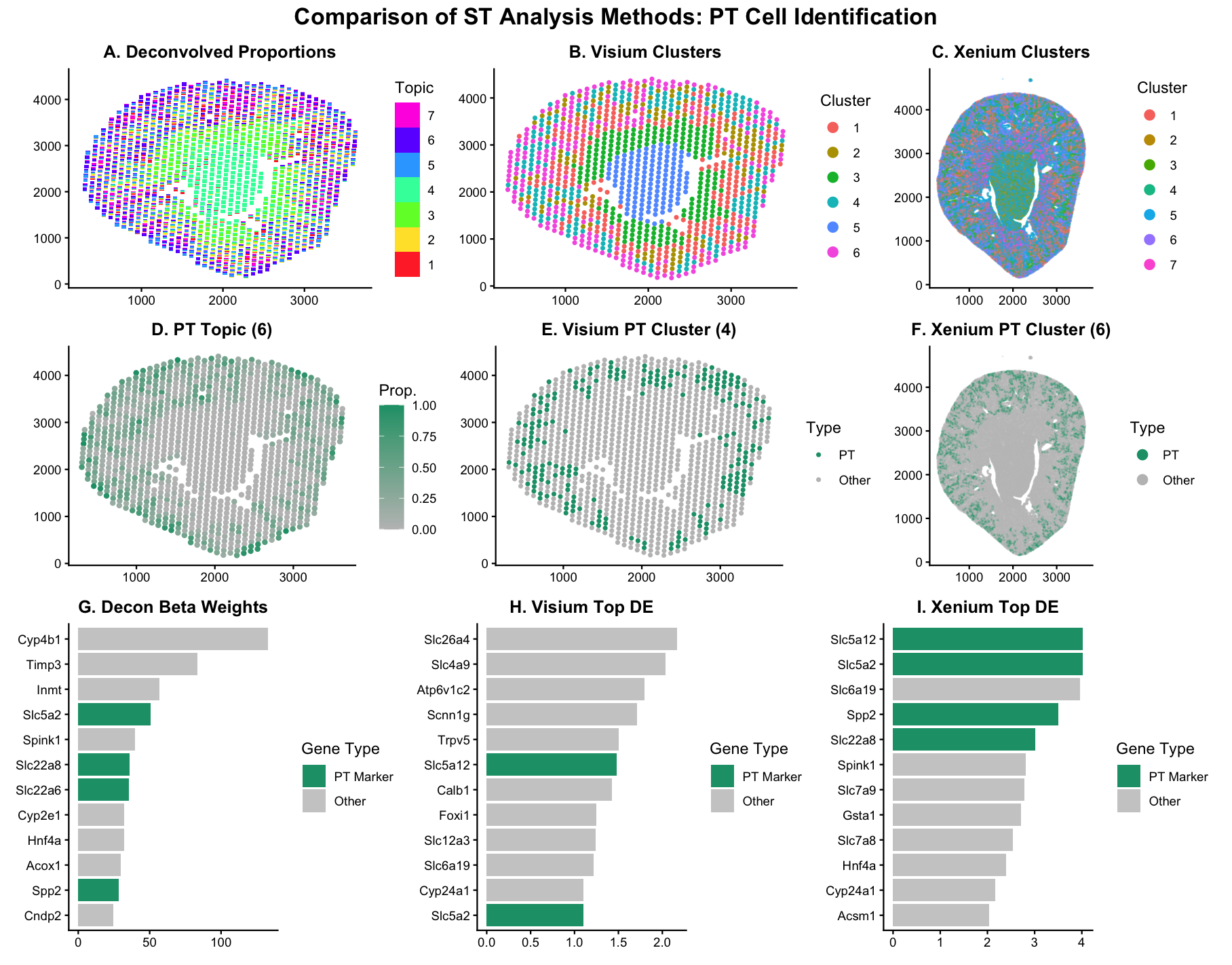
##Description This figure compares three different spatial transcriptomic analysis strategies to identify proximal tubule (PT) cells in mouse kidney tissue using both Visium and Xenium data. From HW3 Research I know that PT cells are a major epithelial cell type in the kidney nephron and play a key role in reabsorbing glucose, ions, and other solutes from the filtrate. Because of their specialized transport function, they express characteristic transporter genes such as Slc5a12, Slc5a2, Slc22a6, Lrp2, and Cubn. These markers allow me to define and validate the PT population across different analytical approaches. The top row shows the global structure produced by each method before I focus on any specific cell type. Panel A displays STdeconvolve topic proportions across Visium spots, where each spot is modeled as a mixture of latent topics that represent putative cell types. Panel B shows K-means clustering on Visium data using the first ten principal components. Panel C shows K-means clustering on Xenium data. This row establishes how each method partitions the tissue overall and provides context before isolating PT cells. The middle row isolates the PT population across all methods. For deconvolution, I identified the PT-associated topic as the one with the highest beta weight for Slc5a12. I initially tried using the default multi-topic visualization, but it was difficult to visually isolate the PT topic because all topics were displayed simultaneously with categorical colors. The PT signal was present, but it was not clearly interpretable. To make the biological pattern more obvious, I instead plotted the PT topic proportion directly as a continuous gradient across the tissue. This makes high-proportion regions visually stand out and allows a clearer comparison to clustering results. For clustering in both Visium and Xenium, I defined the PT cluster as the cluster with the highest mean Slc5a12 expression and highlighted it using the same green color across panels to keep the comparison visually consistent. The bottom row compares gene-level results from deconvolution and clustering. Although Slc5a12 was the primary marker I used to identify PT cells in HW3 and HW4, I highlight multiple known PT markers in the differential expression panels rather than relying on a single gene. Defining a cell type based on one marker can be misleading, especially in noisy or mixed-resolution data. Showing enrichment of several canonical PT transporters strengthens confidence that the identified topic or cluster truly represents proximal tubule cells rather than a technical artifact. Overall, I observe strong agreement between deconvolution and clustering in Visium, with similar spatial localization of PT regions. Xenium shows sharper and more precise boundaries due to its single-cell resolution, but the underlying biological pattern is consistent across methods and platforms.
Note: References and prior AI prompts from HW3 and HW4 are not explicitly restated here, but framework builds directly on that earlier work. Only the new AI prompts used specifically for visualization structure and implementation details in this assignment are documented in the code below.
##Code
1
2
3
4
5
6
7
8
9
10
11
12
13
14
15
16
17
18
19
20
21
22
23
24
25
26
27
28
29
30
31
32
33
34
35
36
37
38
39
40
41
42
43
44
45
46
47
48
49
50
51
52
53
54
55
56
57
58
59
60
61
62
63
64
65
66
67
68
69
70
71
72
73
74
75
76
77
78
79
80
81
82
83
84
85
86
87
88
89
90
91
92
93
94
95
96
97
98
99
100
101
102
103
104
105
106
107
108
109
110
111
112
113
114
115
116
117
118
119
120
121
122
123
124
125
126
127
128
129
130
131
132
133
134
135
136
137
138
139
140
141
142
143
144
145
146
147
148
149
150
151
152
153
154
155
156
157
158
159
160
161
162
163
164
165
166
167
168
169
170
171
172
173
174
175
176
177
178
179
180
181
182
183
184
185
186
187
188
rm(list = ls())
graphics.off()
set.seed(42)

library(STdeconvolve)
library(ggplot2)
library(dplyr)
library(patchwork)
library(scatterbar)

# load visium and xenium datasets
vis <- read.csv("~/Desktop/GDV/Visium-IRI-ShamR_matrix.csv.gz", check.names = FALSE)
xen <- read.csv("~/Desktop/GDV/Xenium-IRI-ShamR_matrix.csv", check.names = FALSE)

pos_vis <- vis[, c("x","y")]
rownames(pos_vis) <- vis[[1]]
gexp_vis <- as.matrix(vis[, 4:ncol(vis)])
rownames(gexp_vis) <- vis[[1]]

pos_xen <- xen[, c("x","y")]
rownames(pos_xen) <- xen[[1]]
gexp_xen <- as.matrix(xen[, 4:ncol(xen)])
rownames(gexp_xen) <- xen[[1]]

# subset visium to xenium gene panel so comparison is fair
xen_genes <- colnames(xen)[4:ncol(xen)]
common <- intersect(colnames(gexp_vis), xen_genes)
gexp_vis_sub <- gexp_vis[, common, drop = FALSE]

# normalize counts and log-transform
lib_vis <- rowSums(gexp_vis_sub)
lib_vis[lib_vis == 0] <- 1
mat_vis <- log10((gexp_vis_sub / lib_vis) * 1e6 + 1)

lib_xen <- rowSums(gexp_xen)
lib_xen[lib_xen == 0] <- 1
mat_xen <- log10((gexp_xen / lib_xen) * 1e6 + 1)

# run STdeconvolve on visium spots
#Help from AI. Prompt: "Show minimal code to run STdeconvolve at K topics,
#extract theta (spot proportions) and beta (topic gene weights)."
K_decon <- 7
ldas <- fitLDA(gexp_vis_sub, Ks = K_decon)
optLDA <- optimalModel(models = ldas, opt = as.character(K_decon))
res <- getBetaTheta(optLDA, perc.filt = 0.05, betaScale = 1000)

theta_vis <- res$theta
beta_vis <- res$beta

# identify PT topic using Slc5a12
marker_gene <- "Slc5a12"
topic_pct_idx <- which.max(beta_vis[, marker_gene])
topic_name_pct <- rownames(beta_vis)[topic_pct_idx]

# PCA + kmeans clustering
pc_vis <- prcomp(mat_vis, center = TRUE)$x[, 1:10]
pc_xen <- prcomp(mat_xen, center = TRUE)$x[, 1:10]

cl_vis <- factor(kmeans(pc_vis, centers = 6, nstart = 50)$cluster)
cl_xen <- factor(kmeans(pc_xen, centers = 7, nstart = 50)$cluster)

# define PT cluster as cluster with highest mean Slc5a12
pct_cluster_vis <- levels(cl_vis)[which.max(
  sapply(levels(cl_vis), function(k) mean(mat_vis[cl_vis == k, marker_gene]))
)]

pct_cluster_xen <- levels(cl_xen)[which.max(
  sapply(levels(cl_xen), function(k) mean(mat_xen[cl_xen == k, marker_gene]))
)]

# simple styling
COL_PT <- "#1B9E77"
COL_BACK <- "grey75"
PT_MARKERS <- c("Slc5a2","Slc5a12","Slc22a6","Slc22a8","Lrp2","Cubn","Spp2")

base_theme <- theme_classic(base_size = 11) +
  theme(
    plot.title = element_text(face = "bold", size = 12, hjust = 0.5),
    axis.title = element_blank()
  )

# A decon proportions
pA <- scatterbar(as.data.frame(theta_vis), pos_vis, padding_x = 40, padding_y = 40) +
  labs(title = "A. Deconvolved Proportions", fill = "Topic") +
  base_theme

# B visium clusters
pB <- ggplot(as.data.frame(pos_vis), aes(x, y, color = cl_vis)) +
  geom_point(size = 0.9) +
  labs(title = "B. Visium Clusters", color = "Cluster") +
  base_theme +
  guides(color = guide_legend(override.aes = list(size = 3)))

# C xenium clusters
#Help from AI. Prompt: "When plotted points are extremely small,
#increase legend symbol size using guide_legend override."
pC <- ggplot(as.data.frame(pos_xen), aes(x, y, color = cl_xen)) +
  geom_point(size = 0.01, alpha = 0.2) +
  coord_fixed() +
  labs(title = "C. Xenium Clusters", color = "Cluster") +
  base_theme +
  guides(color = guide_legend(override.aes = list(size = 3, alpha = 1)))

# D PT topic proportions using manual gradient
#Help from AI. Prompt: "Instead of plotting all topics at once,
#show only one STdeconvolve topic proportion as a gradient map."
df_d <- as.data.frame(pos_vis)
df_d$Proportion <- theta_vis[, topic_name_pct]

pD <- ggplot(df_d, aes(x, y, color = Proportion)) +
  geom_point(size = 1.2) +
  scale_color_gradient(low = COL_BACK, high = COL_PT) +
  labs(title = paste0("D. PT Topic (", topic_name_pct, ")"), color = "Prop.") +
  base_theme

# E visium PT cluster
pE <- ggplot(as.data.frame(pos_vis),
             aes(x, y, color = factor(cl_vis == pct_cluster_vis,
                                      levels = c(TRUE, FALSE)))) +
  geom_point(size = 0.9) +
  scale_color_manual(values = c("TRUE" = COL_PT, "FALSE" = COL_BACK),
                     labels = c("PT", "Other")) +
  labs(title = paste0("E. Visium PT Cluster (", pct_cluster_vis, ")"),
       color = "Type") +
  base_theme

# F xenium PT cluster
pF <- ggplot(as.data.frame(pos_xen),
             aes(x, y, color = factor(cl_xen == pct_cluster_xen,
                                      levels = c(TRUE, FALSE)))) +
  geom_point(size = 0.01, alpha = 0.2) +
  coord_fixed() +
  scale_color_manual(values = c("TRUE" = COL_PT, "FALSE" = COL_BACK),
                     labels = c("PT", "Other")) +
  labs(title = paste0("F. Xenium PT Cluster (", pct_cluster_xen, ")"),
       color = "Type") +
  base_theme +
  guides(color = guide_legend(override.aes = list(size = 3, alpha = 1)))

# gene ranking helper
prep_bar <- function(df, title, y_lab) {
  df$IsPT <- factor(ifelse(df$gene %in% PT_MARKERS,
                           "PT Marker", "Other"),
                    levels = c("PT Marker", "Other"))
  ggplot(df, aes(reorder(gene, val), val, fill = IsPT)) +
    geom_col() +
    coord_flip() +
    scale_fill_manual(values = c("PT Marker" = COL_PT,
                                 "Other" = "grey80")) +
    labs(title = title, x = NULL, y = y_lab, fill = "Gene Type") +
    base_theme
}

# G decon beta weights
df_g <- data.frame(
  gene = names(head(sort(beta_vis[topic_pct_idx, ], TRUE), 12)),
  val = as.numeric(head(sort(beta_vis[topic_pct_idx, ], TRUE), 12))
)
pG <- prep_bar(df_g, "G. Decon Beta Weights", "Weight")

#Help from AI. Prompt: "Compute a simple differential-like ranking
#by subtracting mean expression in other clusters from target cluster."
rank_df <- function(mat, cl, target) {
  val <- colMeans(mat[cl == target, , drop = FALSE]) -
    colMeans(mat[cl != target, , drop = FALSE])
  data.frame(gene = names(val), val = as.numeric(val)) %>%
    arrange(desc(val)) %>%
    head(12)
}

pH <- prep_bar(rank_df(mat_vis, cl_vis, pct_cluster_vis),
               "H. Visium Top DE", "Log2FC")

pI <- prep_bar(rank_df(mat_xen, cl_xen, pct_cluster_xen),
               "I. Xenium Top DE", "Log2FC")

# assemble final figure
final <- (pA | pB | pC) /
  (pD | pE | pF) /
  (pG | pH | pI) +
  plot_layout(heights = c(1, 1, 1.4)) +
  plot_annotation(
    title = "Comparison of ST Analysis Methods: PT Cell Identification",
    theme = theme(plot.title = element_text(size = 16, face = "bold", hjust = 0.5))
  )

final