Characterizing mPOA cell-type heterogeneity with spatial bootstrapping

In this tutorial, we will use SEraster to rasterize the mouse medial preoptic region dataset assayed by MERFISH to demonstrate how tissue section size affects cell-type proportions estimates.

Load libraries

suppressMessages(library(SpatialExperiment))
suppressMessages(library(SEraster))
suppressMessages(library(Matrix))
suppressMessages(library(ggplot2))

One tissue sample of the MERFISH mPOA (bregma -0.29 slice from a female naive animal) dataset is already formatted as a SpatialExperiment object and is available in the SEraster package. We will use this preprocessed dataset in this tutorial (https://jef.works/`SEraster`/reference/merfish_mousePOA.html).

Load dataset

data("merfish_mousePOA")
class(merfish_mousePOA)

## [1] "SpatialExperiment"
## attr(,"package")
## [1] "SpatialExperiment"

Visualize cell-type annotations

First, let’s grab the cell-type annotations from the SpatialExperiment object.

ct <- merfish_mousePOA$celltype; names(ct) <- colnames(merfish_mousePOA)
ct <- as.factor(ct)
head(ct)
length(ct)
length(levels(ct))

## 6d6b1d59-6f3b-4a9d-b5a4-8c8b073ae025 76200644-c14a-4cfa-8752-2a02e5f10d20 
##                          OD Mature 2                        OD Immature 1 
## 6b08ca36-b395-415a-bb34-d7b67550c35d b9cb9cfb-fff7-426e-8c36-18fe428ca156 
##                           Inhibitory                           Excitatory 
## 982cc0fc-6d11-4dc4-9ffc-c8c0cee48e6d ee13ce4c-adf8-4602-9a21-23fdf91d28e0 
##                          OD Mature 2                           Inhibitory 
## 16 Levels: Ambiguous Astrocyte Endothelial 1 Endothelial 2 ... Pericytes
## [1] 6509
## [1] 16

Next, we can use ggplot2 to visualize the cell-type annotations in this tissue section of around 6500 cells comprising 16 cell-types.

## plot
suppressMessages(library(ggplot2))
pos <- spatialCoords(merfish_mousePOA)
df <- data.frame(pos, ct = ct)
ggplot(df, aes(x = x, y = y, color = ct)) +
  coord_fixed() +
  geom_point(size = 0.01) +
  theme_bw()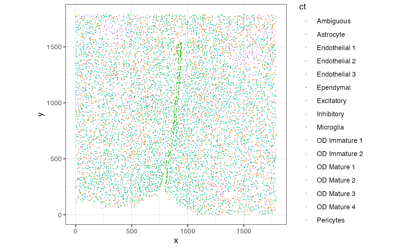

To estimate the cell-type proportions in the whole tissue, we can count the number of each cell-type, divide by the total number of cells and multiply by 100. From this estimation, we see that approximately 30.9% of the cells are Inhibitory, 20.3% are Excitatory, 15.2% are Ambigious, and so forth.

globalEstimate <- table(ct)/length(ct)*100
sort(globalEstimate, decreasing = TRUE)

## ct
##    Inhibitory    Excitatory     Ambiguous     Astrocyte Endothelial 1 
##   30.92640959   20.26424950   15.24043632   11.72223076    5.56153019 
##   OD Mature 2 OD Immature 1     Ependymal     Microglia Endothelial 3 
##    4.04055923    3.36457213    3.10339530    2.07405131    1.62851436 
##     Pericytes   OD Mature 1 Endothelial 2   OD Mature 4   OD Mature 3 
##    0.70671378    0.59917038    0.41481026    0.27654018    0.04609003 
## OD Immature 2 
##    0.03072669

Use `SEraster` to create spatial bootstrap samples

To investigate a smaller section of the tissue, we can use SEraster to aggregate cellular information into square or hexagonal pixels at a resolution of your choosing and investigate the cell-type proportions of each pixel.

suppressMessages(library(SEraster))
## rasterize at 200um resolution with hexagons
rastCt <- SEraster::rasterizeCellType(merfish_mousePOA,
                                      col_name = "celltype",
                                      resolution = 200,
                                      fun = "sum",
                                      square = FALSE)
## plot
SEraster::plotRaster(rastCt, name = "Total cells")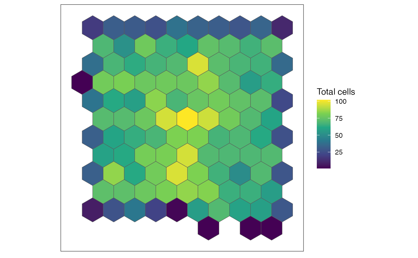

SEraster keeps track of the number of cells in each of these hexagonal pixels and the names of the cells per pixel.

head(colData(rastCt))

## DataFrame with 6 rows and 6 columns
##          num_cell
##         <integer>
## pixel11         1
## pixel14         8
## pixel15        32
## pixel16        32
## pixel17        40
## pixel18        38
##                                                                      cellID_list
##                                                                           <list>
## pixel11                                                   5ade45cb-f1de-45c1-9..
## pixel14 6d6b1d59-6f3b-4a9d-b..,6b08ca36-b395-415a-b..,1baf79d2-f1b7-4a58-9..,...
## pixel15 013f2667-a83f-44b9-a..,dfbf1f48-bdc3-41d8-9..,7320a328-21b2-4c7d-8..,...
## pixel16 2ba4ad43-935e-4dc6-8..,423b0b5d-f22c-464e-a..,29bbf554-d2f2-4ae0-9..,...
## pixel17 6612e339-aabd-4273-a..,ff72229c-5a4f-4dc4-b..,19ff3769-a405-4936-8..,...
## pixel18 1f02025e-2a6d-4b80-9..,c753b3b2-c9aa-4f16-9..,65bc38da-8d3c-4633-8..,...
##                type resolution               geometry   sample_id
##         <character>  <numeric>          <sfc_POLYGON> <character>
## pixel11     hexagon        200 list(c(-100, -200, -..    sample01
## pixel14     hexagon        200 list(c(0, -100, -100..    sample01
## pixel15     hexagon        200 list(c(0, -100, -100..    sample01
## pixel16     hexagon        200 list(c(0, -100, -100..    sample01
## pixel17     hexagon        200 list(c(0, -100, -100..    sample01
## pixel18     hexagon        200 list(c(0, -100, -100..    sample01

## check how many pixels were generated
length(colData(rastCt)$cellID_list)

## [1] 109

## find the hexagonal pixel with the most number of cells
maxCells <- max(rastCt$num_cell) ## 102
pixel <- colnames(rastCt)[colData(rastCt)$num_cell == maxCells]
pixelIdx <- which(colnames(rastCt) == pixel)
print(paste(pixel, " at index ", pixelIdx, " has ", maxCells, " cells."))

## [1] "pixel75  at index  54  has  102  cells."

## double check
colData(rastCt)[pixelIdx,]

## DataFrame with 1 row and 6 columns
##          num_cell
##         <integer>
## pixel75       102
##                                                                      cellID_list
##                                                                           <list>
## pixel75 1022d599-865f-4cf8-9..,c3f95685-61b7-4911-9..,d22dd31f-a6d7-437d-b..,...
##                type resolution               geometry   sample_id
##         <character>  <numeric>          <sfc_POLYGON> <character>
## pixel75     hexagon        200 list(c(900, 800, 800..    sample01

Now, let’s grab the cell-type annotations from the pixel with the highest number of cells and plot the cell-types

## 54th pixel
cells <- colData(rastCt)$cellID_list[[pixelIdx]]
## double check if the number of cells in this pixel matches maxCell
length(cells) == maxCells
## visualize the cells in the 54th pixel
dfsub <- data.frame(pos[cells,], ct = ct[cells])
ggplot(dfsub, aes(x = x, y = y, color = ct)) +
  coord_fixed() +
  geom_point(size = 1.5) +
  theme_bw()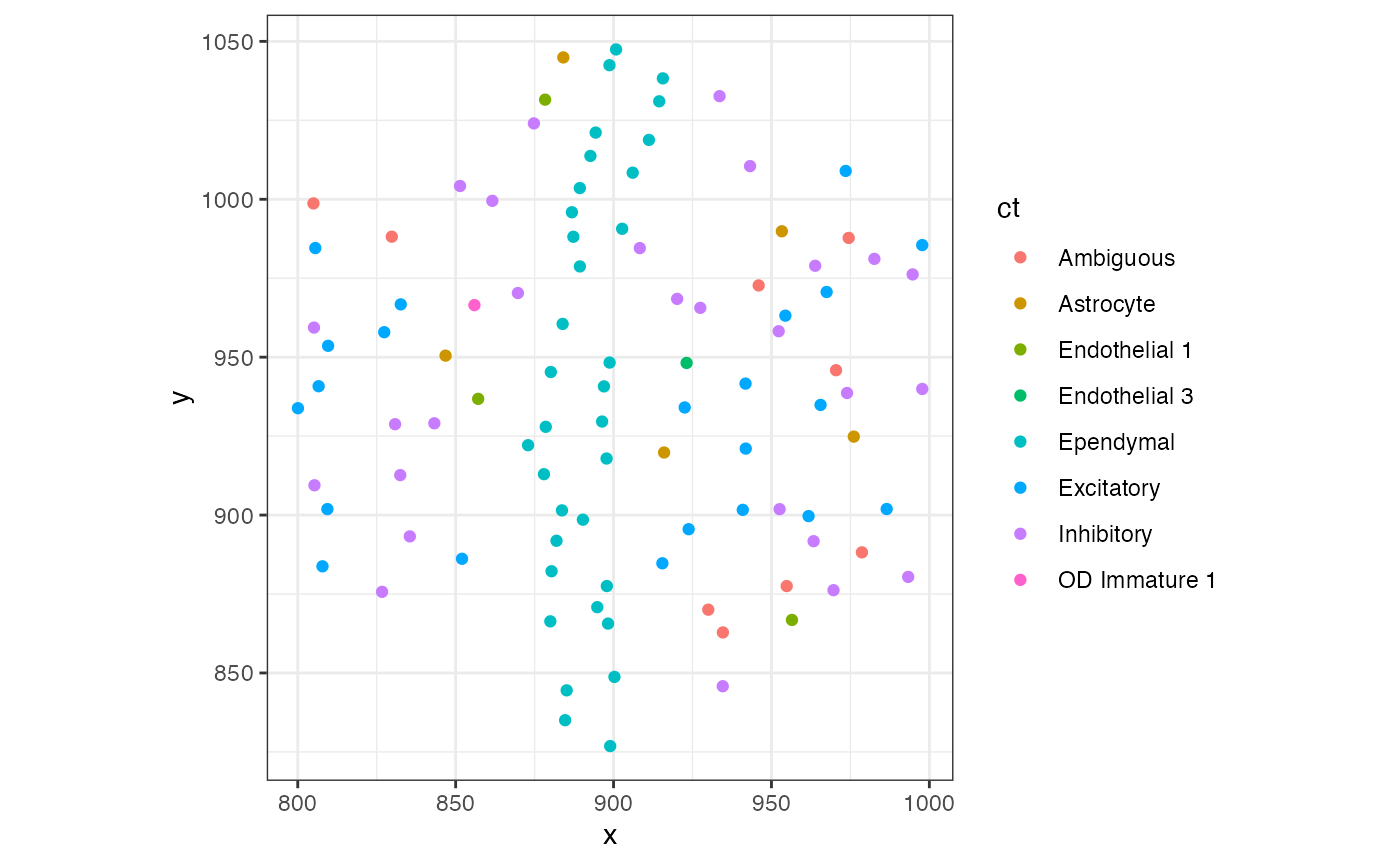

## [1] TRUE

Once again, we can estimate the cell-type proportions. But this time, in pixel 54.

pixelEstimate <- table(ct[cells])/length(ct[cells])*100
sort(pixelEstimate, decreasing = TRUE)

## 
##     Ependymal    Inhibitory    Excitatory     Ambiguous     Astrocyte 
##    33.3333333    26.4705882    21.5686275     8.8235294     4.9019608 
## Endothelial 1 Endothelial 3 OD Immature 1 Endothelial 2     Microglia 
##     2.9411765     0.9803922     0.9803922     0.0000000     0.0000000 
## OD Immature 2   OD Mature 1   OD Mature 2   OD Mature 3   OD Mature 4 
##     0.0000000     0.0000000     0.0000000     0.0000000     0.0000000 
##     Pericytes 
##     0.0000000

We see that approximately 33.3% of the cells in this pixel are Ependymal, 26.5% are Inhibitory, 21.6% are Excitatory, and so forth. This section of the tissue has a relatively high proportion of Ependymal cells compared to the whole tissue. Cell-type proportions for Inhibitory, Excitatory, and Ambiguous are pretty high, consistent with the whole tissue analysis we’ve done earlier.

Now let’s visualize where this pixel is located within the whole tissue by isolating cells not contained in the hexagonal pixel 54.

ctsub <- ct
ctsub[!(names(ctsub) %in% cells)] <- NA
df <- data.frame(pos, ctsub = ctsub)
ggplot(df, aes(x = x, y = y, color = ctsub)) +
  coord_fixed() +
  geom_point(size = 0.1) +
  theme_bw()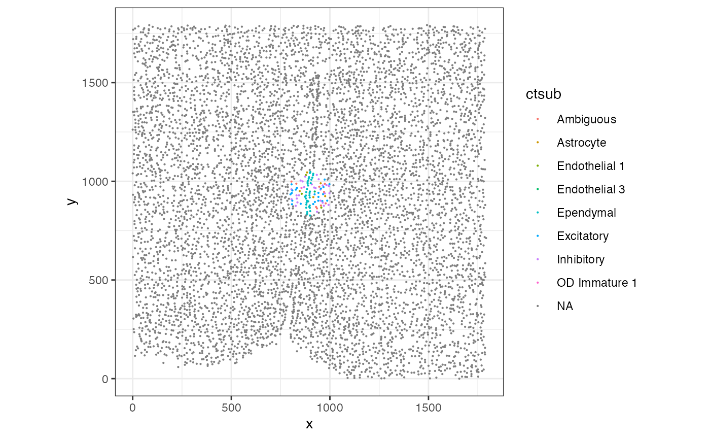

Evaluate stability of cell-type proportions

Let’s assess how good this pixel-based cell-type proportion estimation is in each hexagonal pixel.

## grab list cell IDs for each hexagonal pixel
cellidsPerBiopsy <- colData(rastCt)$cellID_list
names(cellidsPerBiopsy) <- colnames(rastCt)
## loop through and count number of each cell-type
ctprop <- do.call(rbind, lapply(cellidsPerBiopsy, function(i) {
  table(ct[i])
}))
rownames(ctprop) <- names(cellidsPerBiopsy)
head(ctprop)

##         Ambiguous Astrocyte Endothelial 1 Endothelial 2 Endothelial 3 Ependymal
## pixel11         0         0             0             0             0         0
## pixel14         0         3             0             0             0         0
## pixel15        10         3             4             0             0         0
## pixel16         7         2             0             0             0         0
## pixel17         8         1             3             0             0         0
## pixel18         4         0             0             0             1         0
##         Excitatory Inhibitory Microglia OD Immature 1 OD Immature 2 OD Mature 1
## pixel11          0          0         0             0             0           0
## pixel14          0          4         0             0             0           0
## pixel15          6          7         0             1             0           0
## pixel16         10          6         3             1             0           0
## pixel17          2         16         2             2             0           1
## pixel18          6         21         0             3             0           1
##         OD Mature 2 OD Mature 3 OD Mature 4 Pericytes
## pixel11           1           0           0         0
## pixel14           1           0           0         0
## pixel15           1           0           0         0
## pixel16           3           0           0         0
## pixel17           4           0           1         0
## pixel18           2           0           0         0

## divide by total cells per pixel
## and multiple by 100 to make into percents
ctpropNorm <- ctprop/rowSums(ctprop)*100
head(rowSums(ctpropNorm)) ## confirm sum is 100

## pixel11 pixel14 pixel15 pixel16 pixel17 pixel18 
##     100     100     100     100     100     100

head(ctpropNorm)

##         Ambiguous Astrocyte Endothelial 1 Endothelial 2 Endothelial 3 Ependymal
## pixel11   0.00000     0.000           0.0             0      0.000000         0
## pixel14   0.00000    37.500           0.0             0      0.000000         0
## pixel15  31.25000     9.375          12.5             0      0.000000         0
## pixel16  21.87500     6.250           0.0             0      0.000000         0
## pixel17  20.00000     2.500           7.5             0      0.000000         0
## pixel18  10.52632     0.000           0.0             0      2.631579         0
##         Excitatory Inhibitory Microglia OD Immature 1 OD Immature 2 OD Mature 1
## pixel11    0.00000    0.00000     0.000      0.000000             0    0.000000
## pixel14    0.00000   50.00000     0.000      0.000000             0    0.000000
## pixel15   18.75000   21.87500     0.000      3.125000             0    0.000000
## pixel16   31.25000   18.75000     9.375      3.125000             0    0.000000
## pixel17    5.00000   40.00000     5.000      5.000000             0    2.500000
## pixel18   15.78947   55.26316     0.000      7.894737             0    2.631579
##         OD Mature 2 OD Mature 3 OD Mature 4 Pericytes
## pixel11  100.000000           0         0.0         0
## pixel14   12.500000           0         0.0         0
## pixel15    3.125000           0         0.0         0
## pixel16    9.375000           0         0.0         0
## pixel17   10.000000           0         2.5         0
## pixel18    5.263158           0         0.0         0

Let’s visualize the resulting cell-type proportions per hexagonal pixel as a stacked barplot

suppressMessages(library(reshape2))
# Melt the data frame to long format
df <- data.frame(ctpropNorm)
df$Sample <- rownames(df)
dfLong <- melt(df, id.vars = "Sample", variable.name = "CellType", value.name = "Proportion")
head(dfLong)

##    Sample  CellType Proportion
## 1 pixel11 Ambiguous    0.00000
## 2 pixel14 Ambiguous    0.00000
## 3 pixel15 Ambiguous   31.25000
## 4 pixel16 Ambiguous   21.87500
## 5 pixel17 Ambiguous   20.00000
## 6 pixel18 Ambiguous   10.52632

## create the stacked barplot using ggplot2
ggplot(dfLong, aes(x = Sample, y = Proportion, fill = CellType)) +
  geom_bar(stat = "identity") +
  labs(title = "Stacked Barplot of Cell Type Proportions",
       x = "Sample",
       y = "Proportion") +
  theme_minimal() + 
  theme(axis.text.x = element_text(angle = 90, vjust = 0.5, hjust=1, size=5))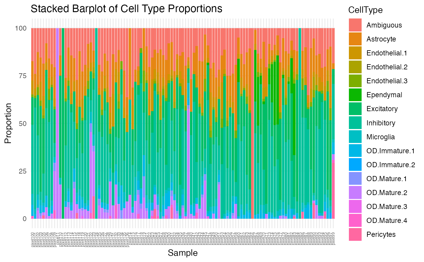

Based on this visualization, we can observe that there is quite a lot of variability in cell-type proportions across each pixel. Let’s find which pixels are the most different from our global cell-type proportion estimate.

diff <- sapply(1:nrow(ctpropNorm), function(i) {
  sum((ctpropNorm[i,]-globalEstimate)^2)
})
names(diff) <- rownames(ctpropNorm)
head(sort(diff, decreasing=TRUE))

##   pixel11   pixel66  pixel111   pixel85  pixel124   pixel38 
## 11004.924  8764.949  7760.186  5627.754  5627.754  4150.976

ctpropNorm['pixel11',]
colData(rastCt)['pixel11',]$num_cell

##     Ambiguous     Astrocyte Endothelial 1 Endothelial 2 Endothelial 3 
##             0             0             0             0             0 
##     Ependymal    Excitatory    Inhibitory     Microglia OD Immature 1 
##             0             0             0             0             0 
## OD Immature 2   OD Mature 1   OD Mature 2   OD Mature 3   OD Mature 4 
##             0             0           100             0             0 
##     Pericytes 
##             0 
## [1] 1

Notice there is only one cell contained in this pixel, and 100% of the pixel of OD Mature 2 cell-type.

pixelIdx <- which(colnames(rastCt) == 'pixel11')
cells <- colData(rastCt)$cellID_list[[pixelIdx]]
## visualize the cells in the 54th pixel
df <- t(data.frame(pos[cells,]))
rownames(df) <- cells
ggplot(df, aes(x = x, y = y, color = ct[cells])) +
  coord_fixed() +
  geom_point(size = 2) +
  theme_bw()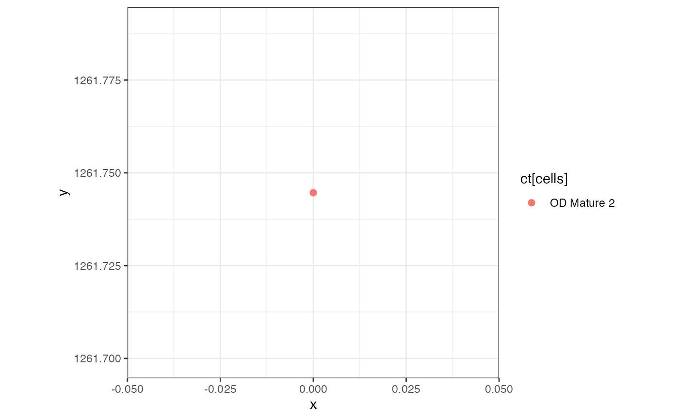

## in whole tissue by setting cells not in hexagonal to NA
ctsub <- ct
ctsub[!(names(ctsub) %in% cells)] <- NA
df <- data.frame(pos, ctsub = ctsub)
ggplot(df, aes(x = x, y = y, color = ctsub)) +
  coord_fixed() +
  geom_point(size = 0.5) +
  theme_bw()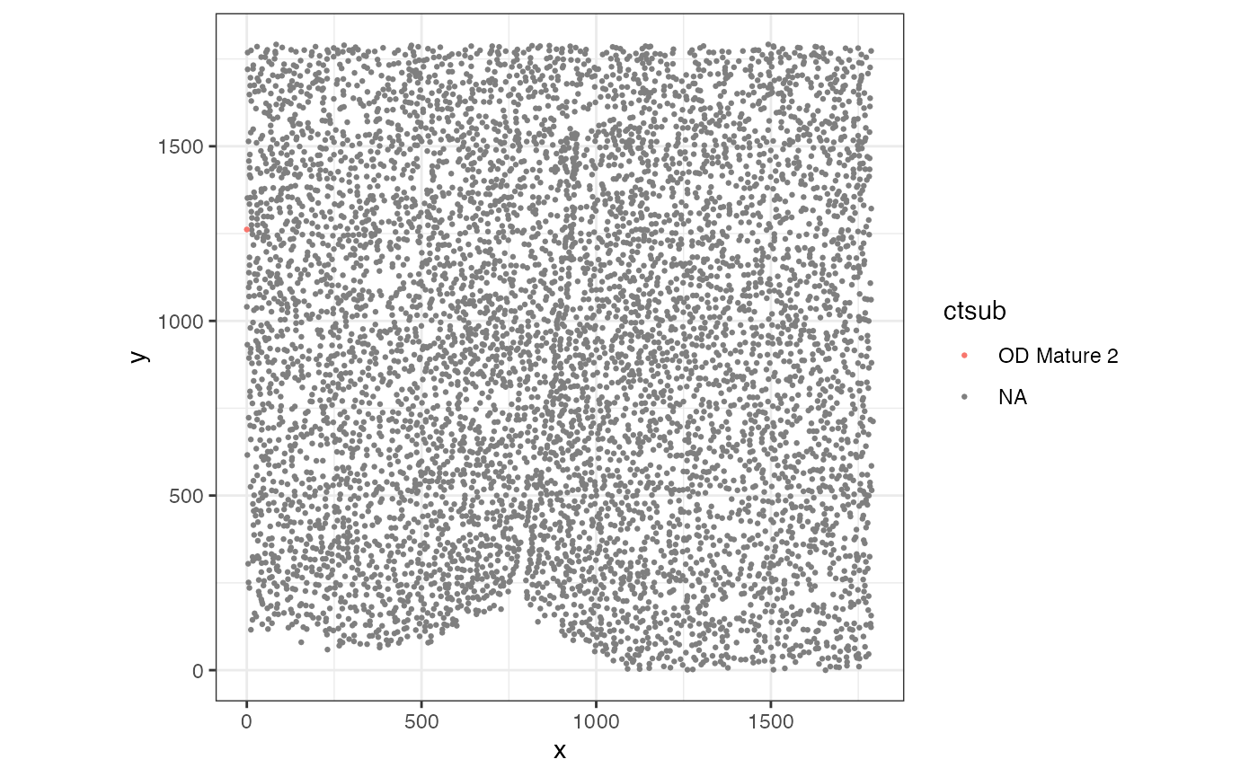

Visually, this pixel is located at the edge of tissue and thus not representative of the whole tissue.

Let’s see the distribution of the number of cells in each hexagonal pixel.

## histogram of number of cells per pixel
hist(colData(rastCt)$num_cell)
## we can set a threshold of only caring about pixels with more than 40 cells
abline(v = 40, col='red')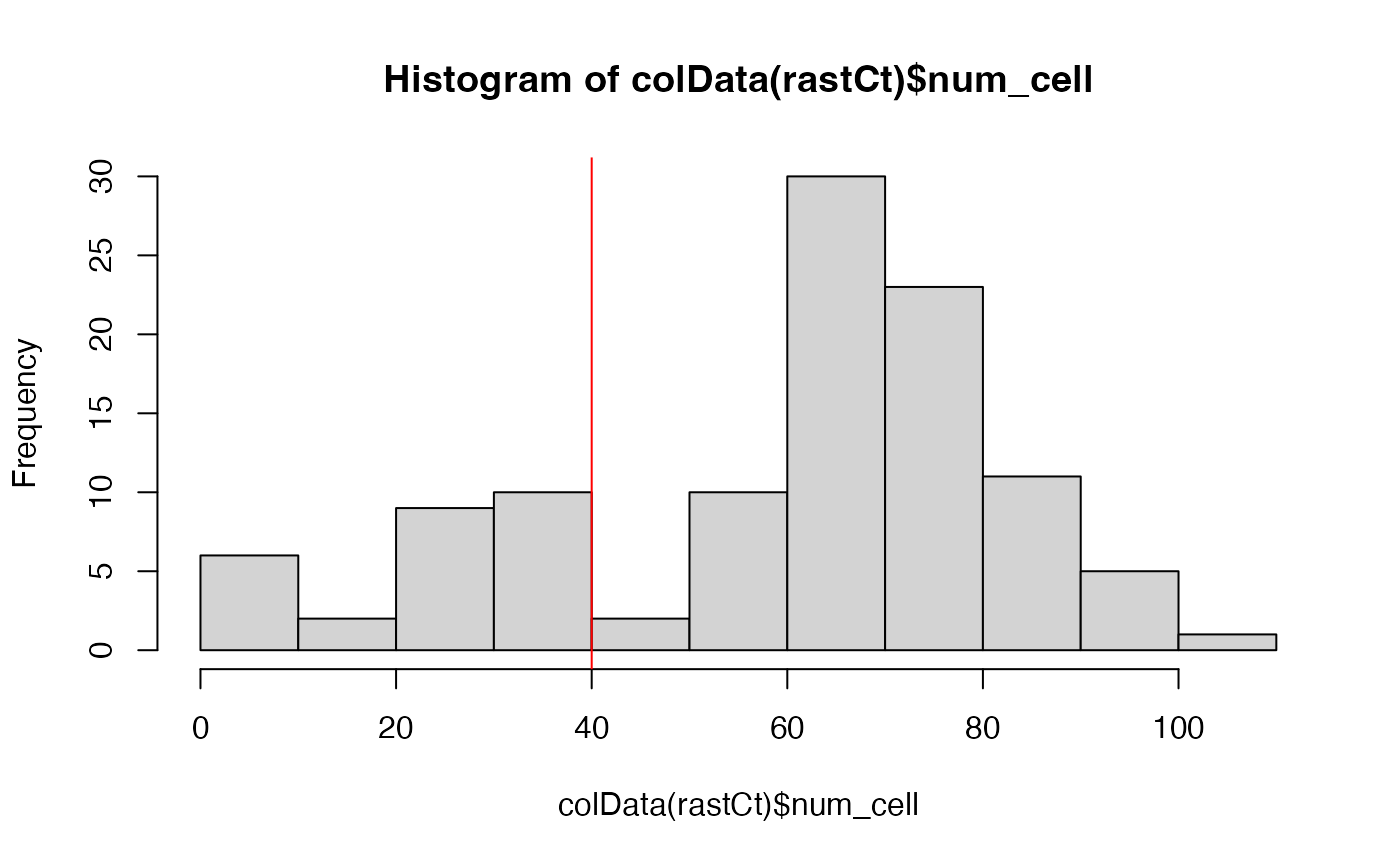

## get pixels with more than 40 cells
goodPixels <- colnames(rastCt)[colData(rastCt)$num_cell > 40]
length(goodPixels)

## [1] 82

head(goodPixels)
goodPixelIdx <- sapply(goodPixels, function(pixel) {
  which(colnames(rastCt) == pixel)
})
head(goodPixelIdx)
## double check
colnames(rastCt)[8] == "pixel21" 
`SEraster`::plotRaster(rastCt[, goodPixelIdx], name = "Total Cells")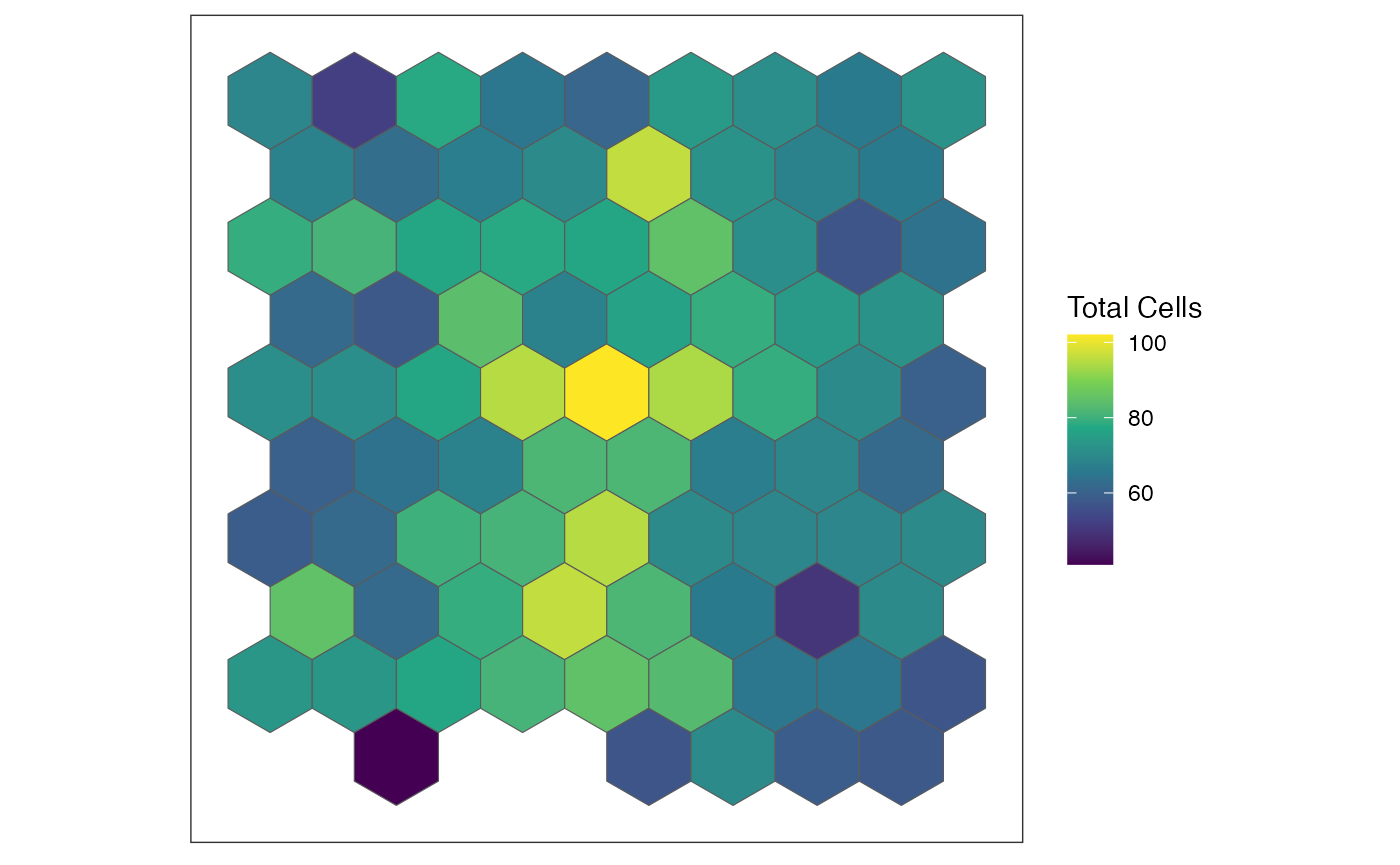

## [1] "pixel21" "pixel22" "pixel23" "pixel24" "pixel25" "pixel28"
## pixel21 pixel22 pixel23 pixel24 pixel25 pixel28 
##       8       9      10      11      12      14 
## [1] TRUE

Now, let’s look at the cell-type proportions for the good pixels we selected.

## just look at ctpropNorm for good pixels
df <- data.frame(ctpropNorm[goodPixelIdx,])
df$Sample <- rownames(df)
dfLong <- melt(df, id.vars = "Sample", variable.name = "CellType", value.name = "Proportion")
ggplot(dfLong, aes(x = Sample, y = Proportion, fill = CellType)) +
  geom_bar(stat = "identity") +
  labs(title = "Stacked Barplot of Cell Type Proportions",
       x = "Sample",
       y = "Proportion") +
  theme_minimal() + 
  theme(axis.text.x = element_text(angle = 90, vjust = 0.5, hjust=1, size=5))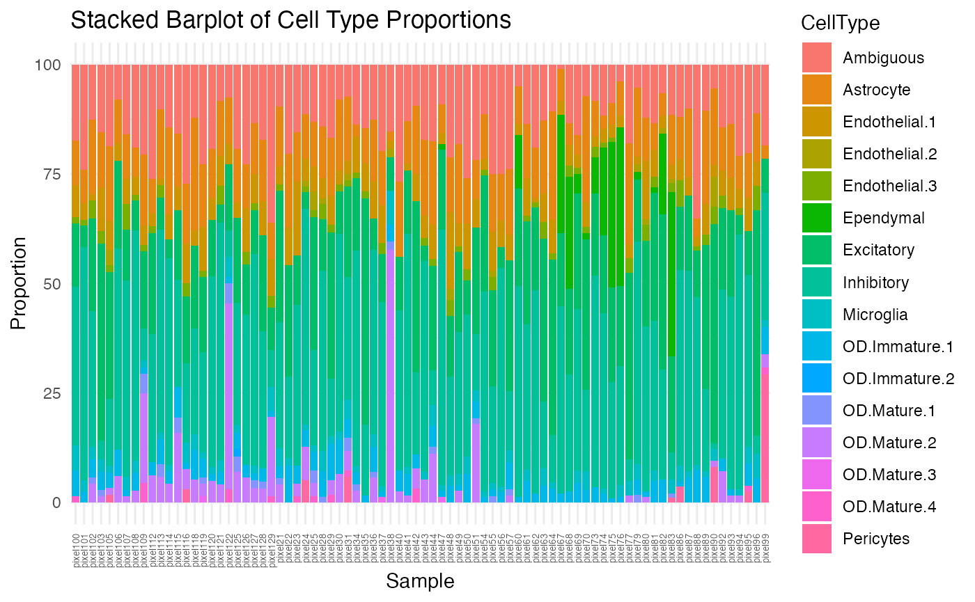

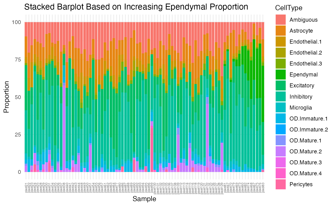
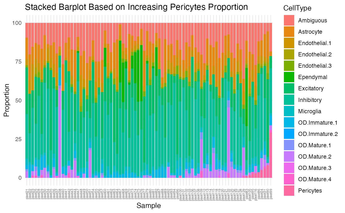
Although better than the previous stacked barplot, there is still some variability, mostly from the Ependymal, OD Mature 2, and Pericytes cell-types. Let’s visualize them based on increasing proportion of each cell-type.

ct.list <- c("Ependymal", "OD.Mature.2", "Pericytes")
for (ct in ct.list) {
  df <- data.frame(ctpropNorm[goodPixelIdx,])
  df$Sample <- rownames(df)
  ## let's create a separate data frame to visualize based on increasing proportion of cell type
  dfLong_ct <- melt(df, id.vars = "Sample", variable.name = "CellType", value.name = "Proportion")
  ## filter dfLong for based on cell type
  df_ct <- dfLong_ct[dfLong_ct$CellType == ct, ]
  ## order the pixels by increasing cell type proportions
  ordered_pixels <- df_ct$Sample[order(df_ct$Proportion)]
  ## convert the sample column to a factor in the with 
  dfLong_ct$Sample <- factor(dfLong_ct$Sample, levels = ordered_pixels)
  show(ggplot(dfLong_ct, aes(x = Sample, y = Proportion, fill = CellType)) +
    geom_bar(stat = "identity") +
    labs(title = paste0("Stacked Barplot Based on Increasing ", ct, " Proportion"),
         x = "Sample",
         y = "Proportion") +
    theme_minimal() + 
    theme(axis.text.x = element_text(angle = 90, vjust = 0.5, hjust=1, size=5)))
}

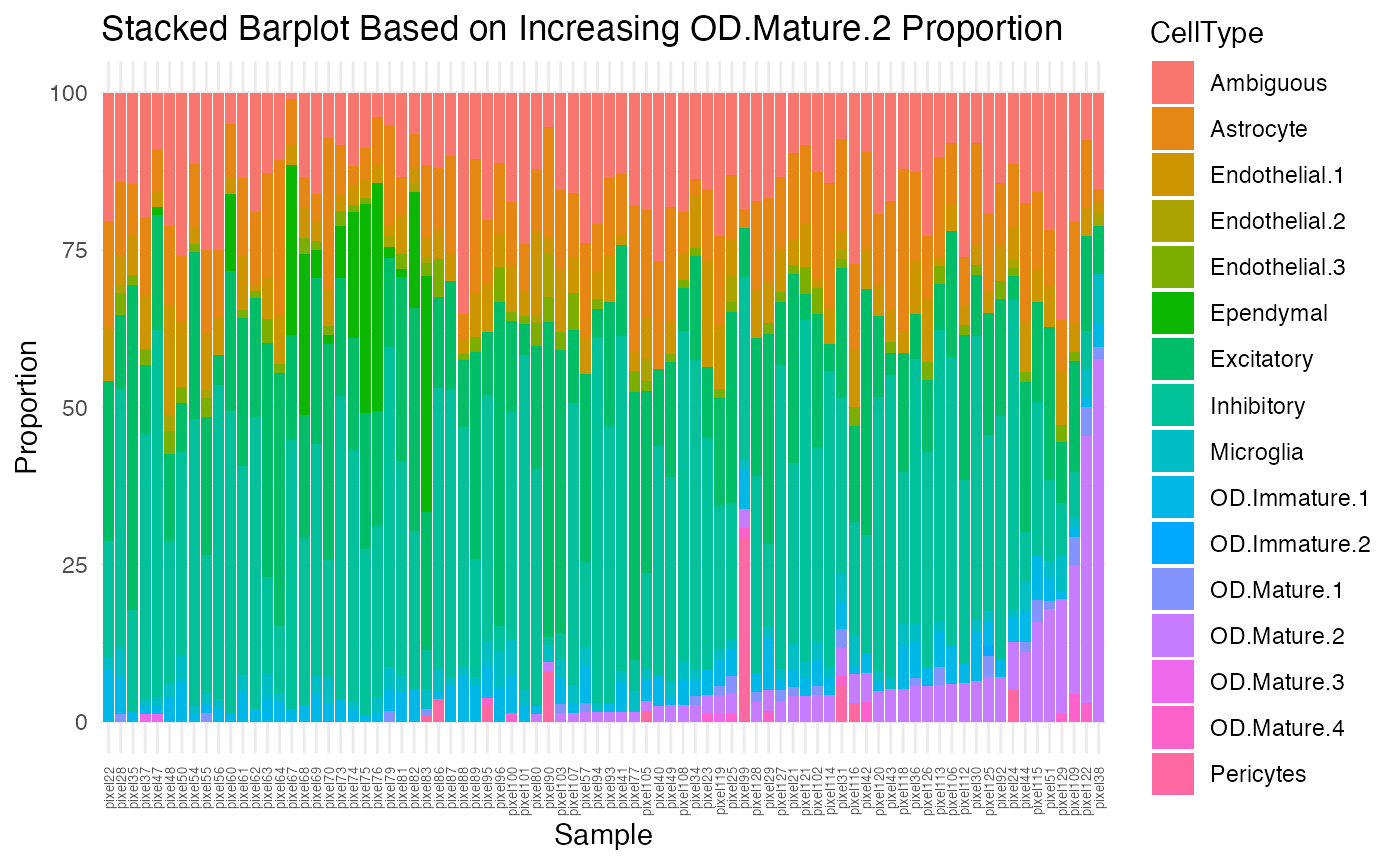
Visualize cell-type specific patterns

The plotRaster function in SEraster allows us to visualize the cell counts by specific cell-types. Let’s try and visualize the spatial distribution of cell counts in these variable cell-types.

ct.list <- c("Ependymal", "OD Mature 2", "Pericytes")
for (ct in ct.list) {
  show(plotRaster(rastCt, plotTitle = ct, feature_name = ct, name = "counts"))
}

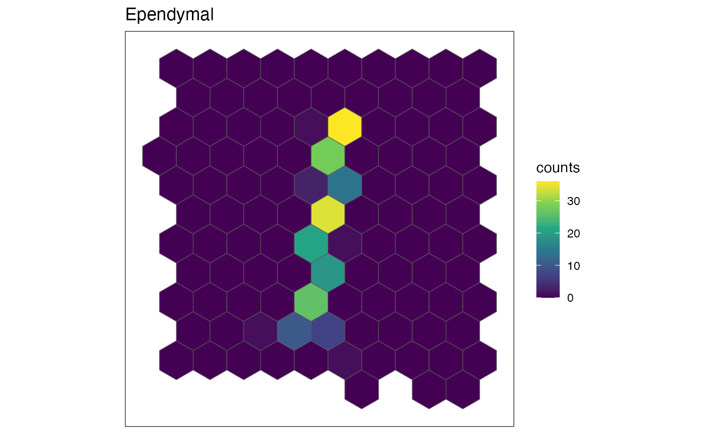
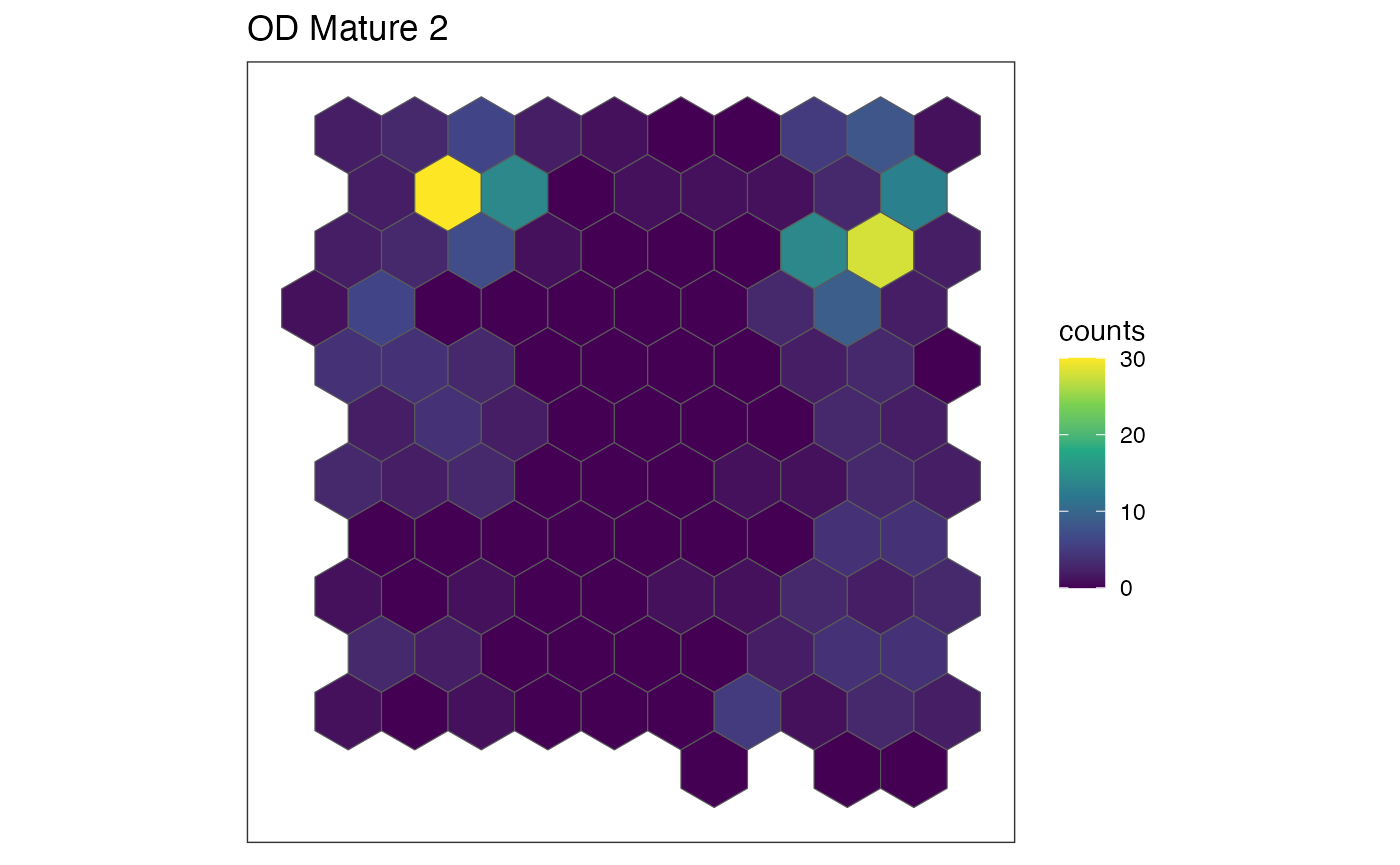
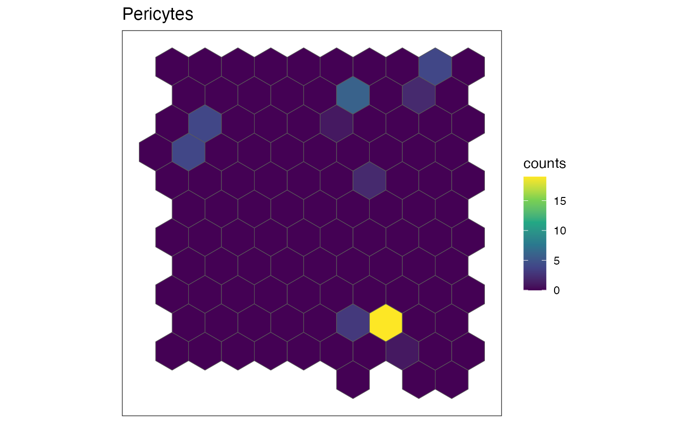
Indeed, we can see that these cell-types are expressed in a spatially variable manner, meaning the pixels containing most of these cell-types are generally not representative of the entire tissue.