spatialCorrelation — spatialCorrelation • STcompare

Function to calculate Pearson's correlation between two spatial datasets. To replace the analytical p-value which results in a high false positive rate for autocorrelated spatial patterns, it calculates empirical p-values from empirical null distributions generated from permuting the datasets and then smoothing to maintain the original degree of autocorrelation

Usage

spatialCorrelation(
  X,
  Y,
  pos,
  nPermutations = 100,
  deltaX = NULL,
  deltaY = NULL,
  maxDistPrctile = 0.25,
  returnPermutations = FALSE,
  nThreads = 1,
  BPPARAM = NULL
)

Arguments

X: numeric or matrix: a 1 x N numeric vector or matrix with N observations
Y: numeric or matrix: a 1 x N numeric vector or matrix with N observations
pos: matrix: a N x 2 matrix array of spatial x,y coordinates of observations
nPermutations: integer or double: number of permutations to generate to build the empirical null distribution. This number will determine the precision of the p-value. Default is 100, such that the smallest p-value is 0.01
deltaX: numeric: A single numeric or a numeric vector for controlling the degree of smoothing in permutations of X. Delta is a proportion calculated by dividing k neighbors by N total observations in X, where k is the number of neighbors in the permutation of X that should be within the radius smoothed by the Gaussian kernel to achieve the amount of autocorrelation present in the original X. If a single delta is not known, a sequence of deltas can be inputted and the best delta will be found such that it minimizes the sum of squares of the residuals between the variogram of the permutation generated from the delta and the variogram of the target. Default is NULL. If no value is supplied for deltaX, seq(0.1,0.9,0.1), the sequence of every 0.1 from 0.1 to 0.9, will be used to find the best delta for X.
deltaY: numeric: A single numeric or numeric vector for controlling the degree of smoothing in permutations of Y. deltaY is like deltaX but for observation in Y instead of X. Default is NULL. If no value is supplied for deltaY, seq(0.1,0.9,0.1), the sequence of every 0.1 from 0.1 to 0.9, will be used to find the best delta for permutations of Y.
maxDistPrctile: numeric: percentile of distances between pixels to use as max distance in when calculating variograms. Default = 0.25. At greater distances the variogram is less precise because there are fewer pairs of points with that distance between them. Therefore, since the goal is to minimize the difference between the variogram of X and those of its permutations, the variogram should be subsetted to the percentile that is more robust.
returnPermutations: logical: FALSE (default) indicate whether the outputted dataframe will have a column with the values of the permutations used to calculate the null correlations and the empirical p-value.
nThreads: integer: Number of threads for parallelization. Default = 1. Inputting this argument when the BPPARAM argument is NULL would set parallel execution back-end to be BiocParallel::MulticoreParam(workers = nThreads). We recommend setting this argument to be the number of cores available (parallel::detectCores(logical = FALSE)). If BPPARAM argument is not NULL, the BPPARAM argument would override nThreads argument.
BPPARAM: BiocParallelParam: Optional additional argument for parallelization. This argument is provided for advanced users of BiocParallel for further flexibility for setting up parallel-execution back-end. Default is NULL. If provided, this is assumed to be an instance of BiocParallelParam.

Value

The output is returned as a data.frame containing the columns:

correlationCoefPearson's correlation coefficient.
pValueNaivethe analytical p-value naively assuming independent observations
pValuePermuteXthe p-value when creating an empirical null from permutations of observations in X
pValuePermuteYthe p-value when creating an empirical null from permutations of observations in Y
deltaStarMedianXthe median delta star (the delta which minimizes the difference between the variogram of the permutation and the variogram of observations) across permutations of X
deltaStarMedianYthe median delta star across permutations of Y
deltaStarXlist of delta star for all permutations of X
deltaStarYlist of delta star for all permutations of Y
nullCorrelationsXcorrelation coefficients for pairing Y and all permutations of X
nullCorrelationsYcorrelation coefficients for pairing X and all permutations of Y
permutationsX(optional) a N x B matrix, where N is the length of X and B is `nPermutations`. Each column is the resulting values of a permutation of X
permutationsY(optional) a N x B matrix, where N is the length of Y and B is `nPermutations`. Each column is the resulting values of a permutation of Y

Examples


data(quakes)

#remove duplicated positions
quakes_data <- quakes[!duplicated(cbind(quakes$lat, quakes$long)),]

cor <- spatialCorrelation(X = quakes_data$depth,
                          Y = quakes_data$mag,
                          pos = cbind(quakes_data$lat, quakes_data$long))
cor
#>     correlationCoef  pValueNaive pValuePermuteX pValuePermuteY deltaStarMedianX
#> cor       -0.230266 1.779041e-13           0.05           0.09              0.8
#>     deltaStarMedianY   deltaStarX   deltaStarY nullCorrelationsX
#> cor              0.5 0.5, 0.6.... 0.6, 0.7....      0.190177....
#>     nullCorrelationsY
#> cor      -0.08056....

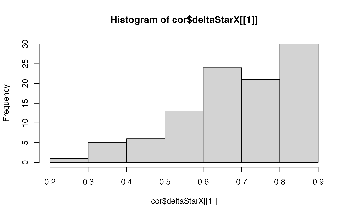
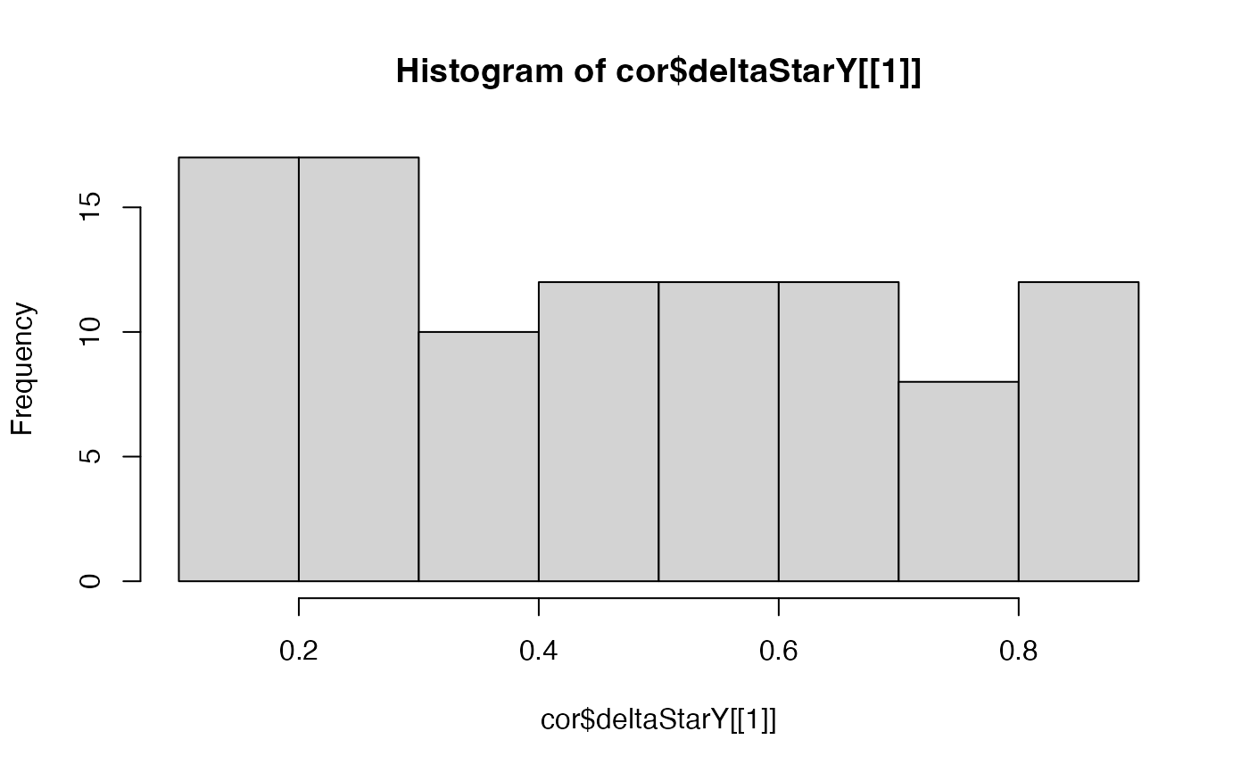
# plot the delta star (the delta which minimizes the difference between the
# variogram of the permutation and the variogram of observations) for all
# permutations to see if clear peak found in the range inputted
hist(cor$deltaStarX[[1]])

hist(cor$deltaStarY[[1]])


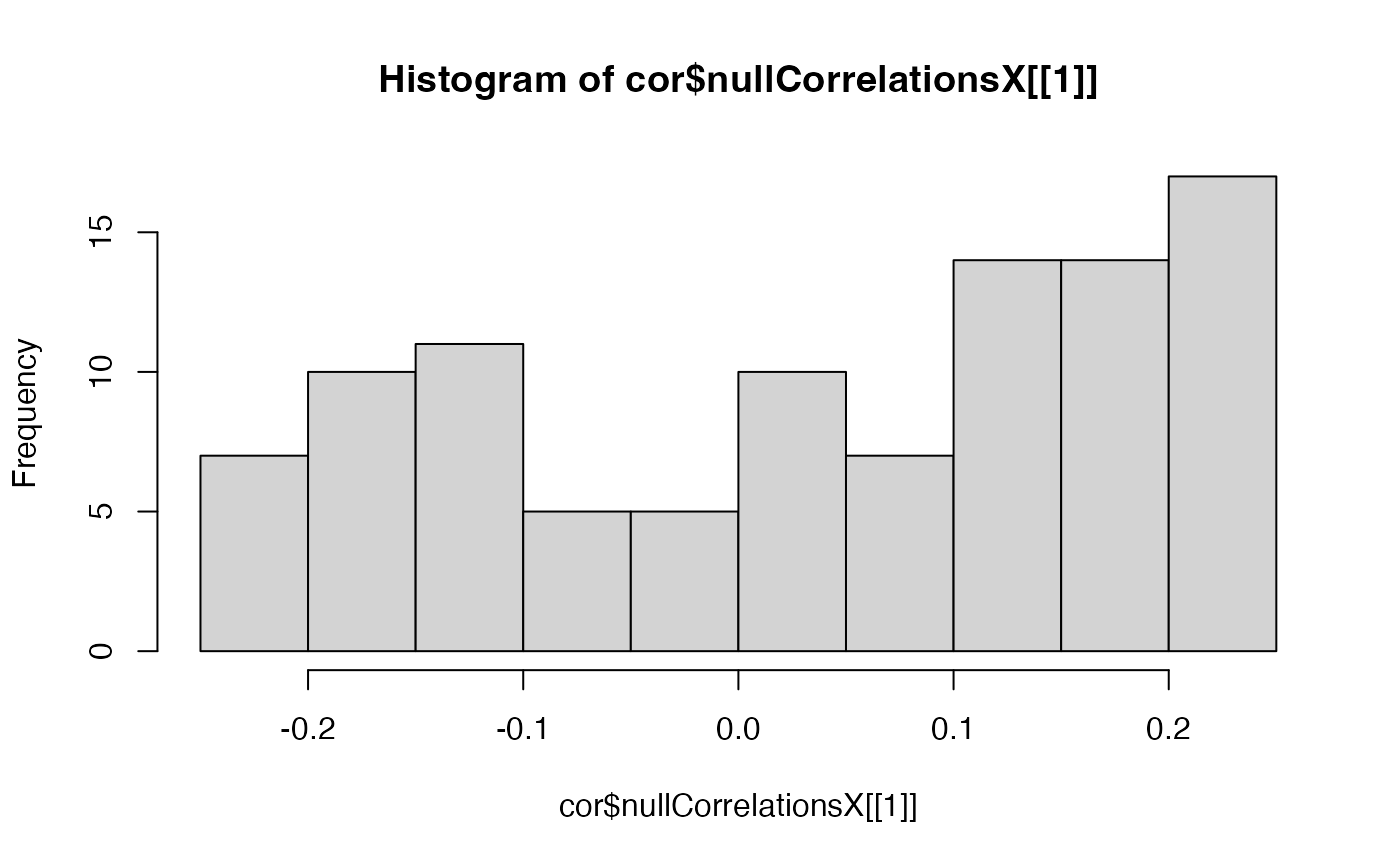
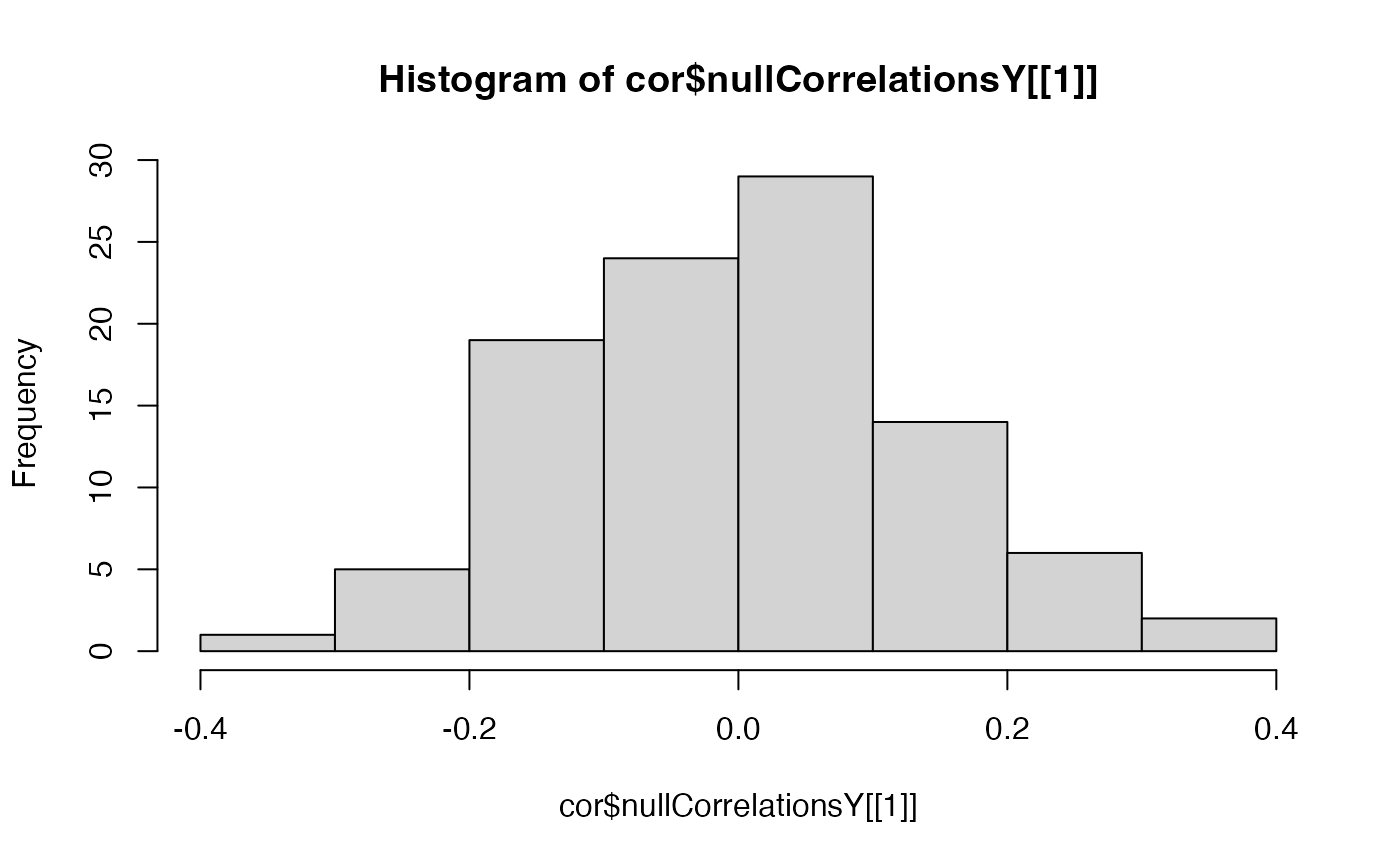
#plot null distribution of correlations to see if normally distributed
hist(cor$nullCorrelationsX[[1]])

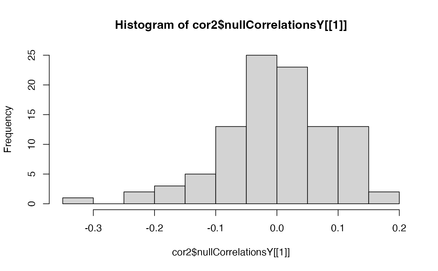
hist(cor$nullCorrelationsY[[1]])


#example of inputting specific range for deltaX and deltaY
cor2 <- spatialCorrelation(X = quakes_data$depth,
                          Y = quakes_data$mag,
                          pos = cbind(quakes_data$lat, quakes_data$long),
                          deltaX = seq(0.05, 0.9, 0.05),
                          deltaY = seq(0.02, 0.5, 0.02))

cor2
#>     correlationCoef  pValueNaive pValuePermuteX pValuePermuteY deltaStarMedianX
#> cor       -0.230266 1.779041e-13           0.04           0.01             0.75
#>     deltaStarMedianY   deltaStarX   deltaStarY nullCorrelationsX
#> cor             0.24 0.9, 0.9.... 0.42, 0.....      -0.17102....
#>     nullCorrelationsY
#> cor      0.060023....

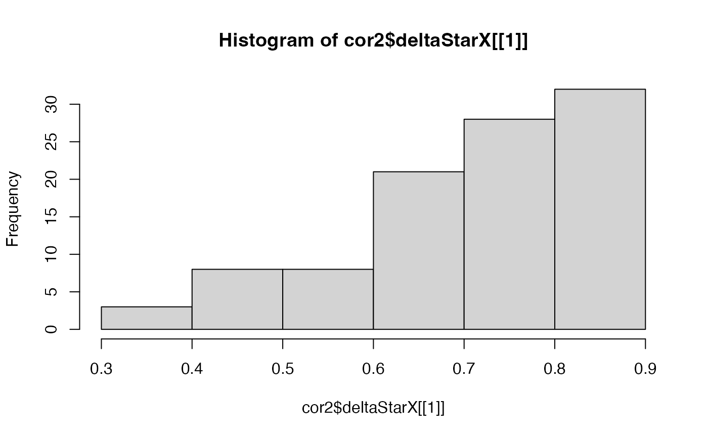
hist(cor2$deltaStarX[[1]])

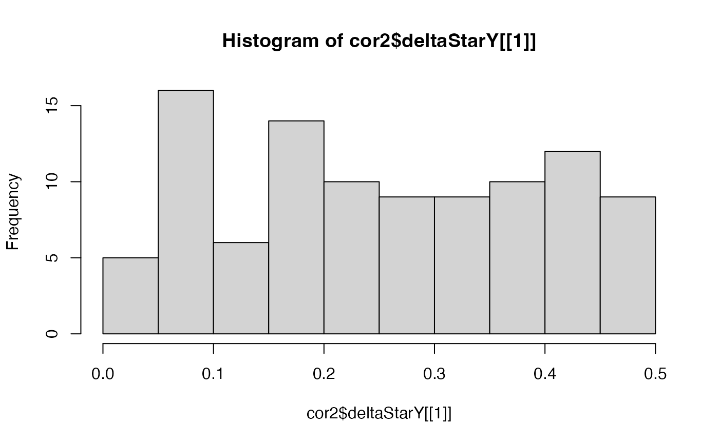
hist(cor2$deltaStarY[[1]])

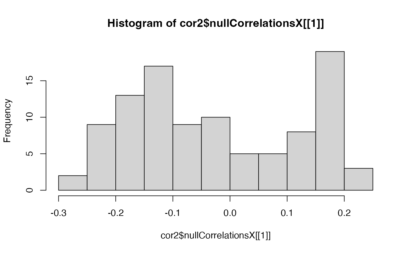
hist(cor2$nullCorrelationsX[[1]])

hist(cor2$nullCorrelationsY[[1]])


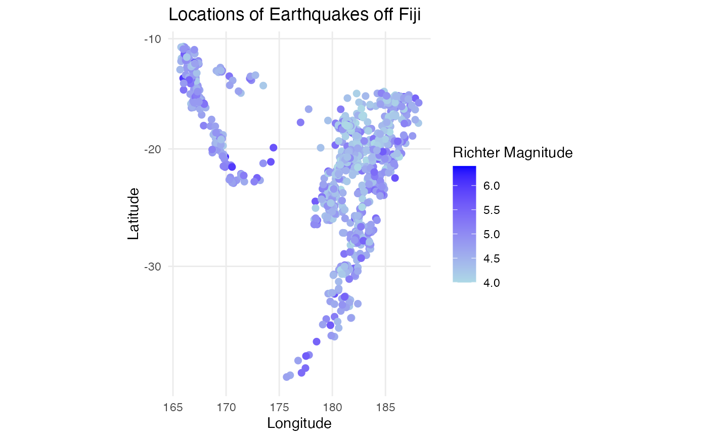
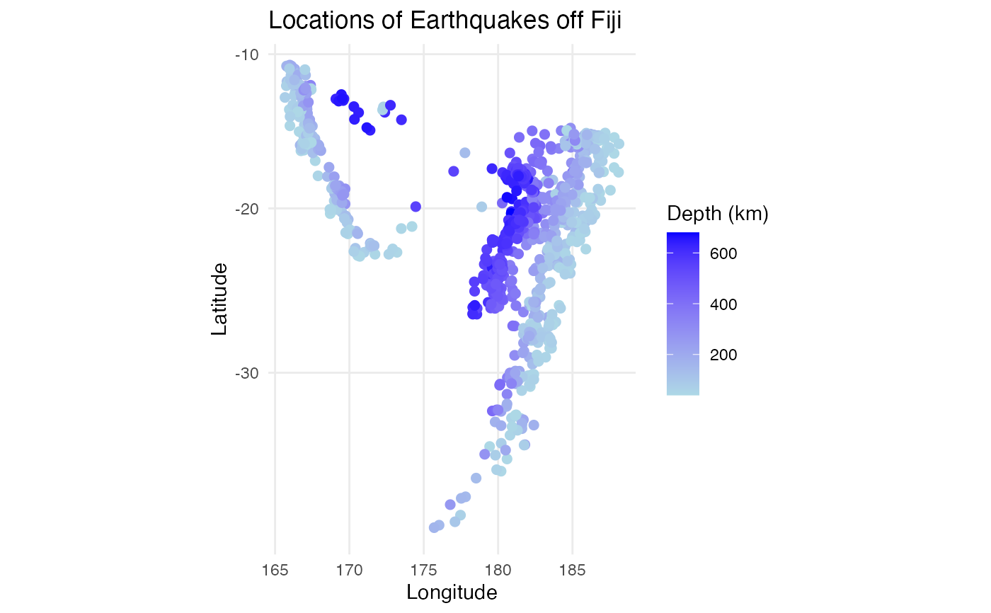
#visualizations of the spatial data to verify negative correlation
library(ggplot2)
p1 <- ggplot2::ggplot(quakes_data,
                      ggplot2::aes(x = long, y = lat, color = depth)) +
ggplot2::geom_point(size = 2) +
  ggplot2::scale_color_gradient(low = "lightblue", high = "blue") +
  ggplot2::labs(title = "Locations of Earthquakes off Fiji",
                x = "Longitude", y = "Latitude",
                color = "Depth (km)") +
  ggplot2::theme_minimal() +
  ggplot2::coord_map()

p2 <- ggplot2::ggplot(quakes_data,
                      ggplot2::aes(x = long, y = lat, color = mag)) +
ggplot2::geom_point(size = 2) +
  ggplot2::scale_color_gradient(low = "lightblue", high = "blue") +
  ggplot2::labs(title = "Locations of Earthquakes off Fiji",
                x = "Longitude", y = "Latitude",
                color = "Richter Magnitude") +
  ggplot2::theme_minimal() +
  ggplot2::coord_map()

p1

p2