Identifying Interesting Cells By Spatial Transcriptomics

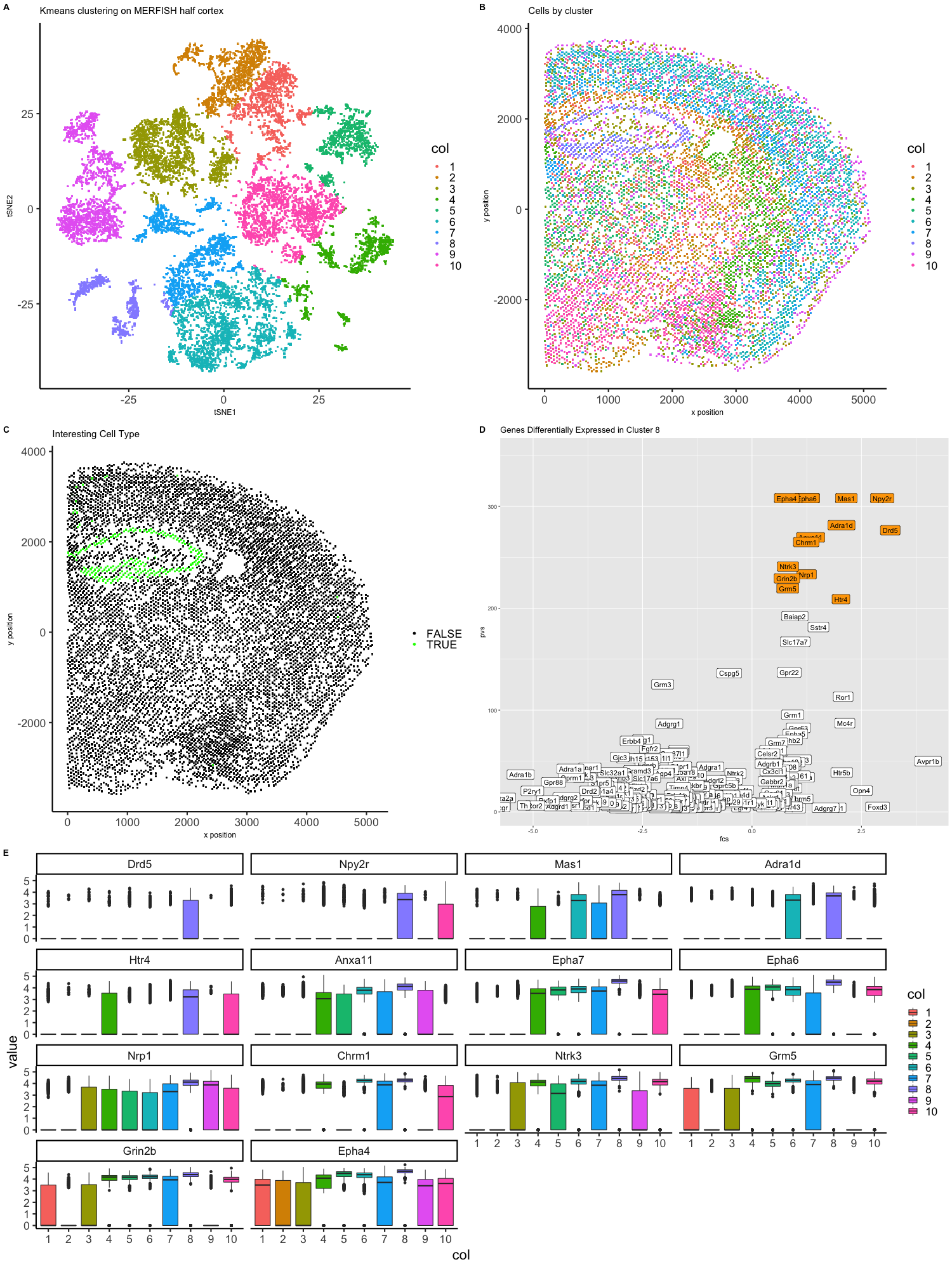
Expression of 483 genes has been measured in 42519 cells in a segment of brain tissue via MERFISH. Each cell position in the tissue sample has also been recorded. Fluorescence intensity has been lognormalized by cell such that each data point is the log10(count) of transcripts for a gene if the total number of transcripts for all genes in that cell was 1 million. To display the data in low dimensional space, tSNE was performed on the first twenty-five principle components from doing PCA on the gene expression matrix. The embedding was then used as variables to group cells by kmeans clustering into ten clusters. The clusters have been visualized on the low dimensional embeddings (Figure A). Additionally, cells were plotted as they appear positionally in the tissue sample and labeled by cluster membership (Figure B). Cells in cluster 8 seem unique in both placement in the tissue and position in tsNE embedding so that cluster was chosen for further analysis (Figure C). Two-sided Wilcox tests were perfomred for each gene to determine if it was differentially expressed bewteen cells in cluster 8 and all other cells. Genes that had statistically signifcant differential expression (adjusted p-value < 0.05) were selected to be inlcuded in a volcano plot with the axes being log2(fold change) and -log10(p-value). Genes that were upregulated in cluster 8 and had the lowest p-values were identified (Figure D). Boxplots were created to show differential expression across the ten clusters for these upregulated genes (Figure E).
Drd5 (Dopamine Receptor D5) is reported in literature to be “anatomically localized to the cortex, hippocampus and limbic system.” (ref 1) The limbic system includes structure such as the amygdala, thalamus, hypothalamus, basal ganglia, and cingulate gyrus. Npy2r (Neuropeptide Y2 receptor) is “widespread in the human central nervous system with particularly dense regions in the hypothalamus and the hippocampus.” (ref 2) Similarly, HTR4 is “highly expressed in the central nervous system, particularly in limbic structures.” (ref 3)
From the differential expression analysis, literature review and anatomical positioning, my best guess is that cells in cluster 8 are part of the hypothalamus, but they could be part of other limbic structures.
References:
- https://www.psychiatrictimes.com/view/dopamine-receptors-human-brain
- https://www.diva-portal.org/smash/get/diva2:432641/FULLTEXT01.pdf
- https://respiratory-research.biomedcentral.com/articles/10.1186/1465-9921-14-77
#load libraries
library(Rtsne)
library(ggplot2)
library(scattermore)
library(gridExtra)
library(reshape2)
library(cowplot)
library(Hmisc)
library(tidyr)

#load MERFISH data
data <- read.csv('~/Dropbox/JHU/Courses/genomic-data-visualization/data/MERFISH_Slice2Replicate2_halfcortex.csv.gz')

#downsample to 15000
set.seed(0)
vi <- sample(data[,1],15000)
ds <- data[data$X %in% vi,]

#make matrix of position
pos <- ds[, c('x','y')]
rownames(pos) <- ds[,1]
plot(pos, pch='.')

#make matrix of gene expression data without position
gexp <- ds[, 4:ncol(ds)]
rownames(gexp) <- ds[,1]

#CPM normalize
numgenes <- rowSums(gexp)
normgexp <- gexp/numgenes*1e6

#add pseudocounts to do log
mat <- log10(normgexp+1)

###############
#PCA
set.seed(0)
pcs <-prcomp(mat)
df <- data.frame(x=c(1:100), y=pcs$sdev[1:100])
p <- ggplot(data = df,mapping = aes(x=x,y=y) ) + geom_line() +
  labs(title="Principle Components", x="index", y = "standard deviation")
p

###############
# tSNE
set.seed(0)
emb <- Rtsne(pcs$x[,1:25], dims=2, perplexity = 30)$Y
#emb <- Rtsne(mat, dims=2, perplexity = 30)$Y
rownames(emb) <- rownames(mat)
#head(emb)
#dim(emb)

###############
# kmeans on gene expression
set.seed(0)
#com <- kmeans(mat, centers=10)
com <- kmeans(emb, centers=10)
#com <- kmeans(pcs$x[,1:30], centers=10)

#plot kmeans clusters on tSNE dimensions
dfk <- data.frame(x = emb[,1],
                  y = emb[,2],
                  col = as.factor(com$cluster))
pk <- ggplot(data = dfk,
             mapping = aes(x = x, y = y)) +
  geom_scattermore(mapping = aes(col = col),
                   pointsize=1) +
  theme_classic(base_size=22) +
  labs(title="Kmeans clustering on MERFISH half cortex", x = "tSNE1" , y = "tSNE2") +
  theme(axis.title=element_text(size=12), plot.title = element_text(size=15))
pk

#plot kmeans clusters with cell positions
dfpo <- data.frame(x = pos[,1],
                   y = pos[,2],
                   col = as.factor(com$cluster))
ppo <- ggplot(data = dfpo, mapping = aes(x = x, y = y)) +
  geom_scattermore(mapping = aes(col = col), pointsize=1) +
  theme_classic(base_size=22) +
  labs(title="Cells by cluster", x = "x position" , y = "y position")+
  theme(axis.title=element_text(size=12), plot.title = element_text(size=15))
ppo

grid.arrange(pk, ppo, ncol=2)

# interested in small grouping that isn't well labeled in clustering

small_data <- mat[c(which(com$cluster==5), which(com$cluster==6)),]
dim(small_data)
#com2 <- kmeans(small_data, centers=2)

###############
#PCA
set.seed(0)
pcs2 <-prcomp(small_data)
df2 <- data.frame(x=c(1:30), y=pcs2$sdev[1:30])
p2 <- ggplot(data = df2,mapping = aes(x=x,y=y) ) + geom_line() +
  labs(title="Principle Components", x="index", y = "standard deviation")
p2


###############
# tSNE
set.seed(0)
emb2 <- Rtsne(pcs2$x[,1:10], dims=2, perplexity = 30)$Y
emb2 <- Rtsne(small_data, dims=2, perplexity = 30)$Y
rownames(emb2) <- rownames(small_data)
#head(emb)
#dim(emb)

###############
# kmeans on gene expression
set.seed(0)
com2 <- kmeans(small_data, centers=3)
#com <- kmeans(emb2, centers=3)
#com <- kmeans(pcs2$x[,1:10], centers=10)


#plot kmeans clusters on tSNE dimensions
dfk <- data.frame(x = emb2[,1],
                  y = emb2[,2],
                  col = as.factor(com2$cluster))
pk <- ggplot(data = dfk,
             mapping = aes(x = x, y = y)) +
  geom_scattermore(mapping = aes(col = col),
                   pointsize=1) +
  theme_classic(base_size=22) +
  labs(title="Kmeans clustering", x = "tSNE1" , y = "tSNE2") +
  theme(axis.title=element_text(size=12), plot.title = element_text(size=15))
pk

#########
# Differential gene expression
# For cluster of interest find which genes are differentially expressed

# store vector of whether cells are in cluster one or two
cluster_int <- com$cluster == 8

## wilcox test on all genes for cells in cluster 3 against all other cells
## save the pvalues
pvs <- sapply(colnames(mat), function(g) {
  x = wilcox.test(mat[cluster_int, g], mat[!cluster_int, g],
                  alternative='two.sided')
  return(x$p.value)
})
## correct for multiple testing
table(p.adjust(pvs) < 0.05)
table(pvs < 0.05)

## calculate fold changes
fcs <- sapply(colnames(mat), function(g) {
  x = mean(mat[cluster_int, g])/mean(mat[!cluster_int, g])
  return(x)
})

# make list of genes differentially expressed in interesting cluster with p-value < 0.05
gl <- names(which(p.adjust(pvs) < 0.05))
gl <- names(sort(fcs[gl], decreasing=TRUE))

# volcano plot only genes differential expressed in interesting cluster with p-value < 0.05
# add pseudocount of 1e-308, numbers smaller than 1e-308 are otherwise set to the limit of the graph
dfv <- data.frame(name = gl,
                  pvs = -log10(pvs + 1e-308)[gl],
                  fcs = log2(fcs)[gl])
pv <- ggplot(dfv, mapping = aes(x=fcs, y=pvs)) +
  geom_point() + geom_label(mapping = aes(label = name)) + ylim(NA,350)

pv
# genes of interest for visual inspection of volcano plot
# -log10(pvs)[gl] > 200 & log2(fcs)[gl] > 0

# make list of genes of interest
gup <- names(which(-log10(pvs)[gl] > 200 & log2(fcs)[gl] > 0))
gup <- names(sort(fcs[gup], decreasing=TRUE))

# remake volcano plot with highest fold change and lowest p-values labeled
dfv2 <- data.frame(name = gl,
                  pvs = -log10(pvs + 1e-308)[gl],
                  fcs = log2(fcs)[gl],
                  group = -log10(pvs)[gl] > 200 & log2(fcs)[gl] > 0)
pv2 <- ggplot(dfv2, mapping = aes(x=fcs, y=pvs)) +
  geom_point() + geom_label(mapping = aes(label = name, fill=group)) + ylim(NA,350) +
  scale_fill_manual(values = c("white","orange")) + theme(legend.position = "none") +
  labs(title="Genes Differentially Expressed in Cluster 8")
pv2


# Box plots by cluster for genes of interest
dfcs <- reshape2::melt(
  data.frame(id=rownames(mat),
             mat[, gup],
             col=as.factor(com$cluster)))

pcs <- ggplot(data = dfcs,
              mapping = aes(x=col, y=value, fill=col)) +
  geom_boxplot() +
  theme_classic(base_size=22) +
  facet_wrap(~ variable)
pcs

#plot position of cells colored by interesting cluster
dfpo2 <- data.frame(x = pos[,1],
                   y = pos[,2],
                   celltype = cluster_int)
ppo2 <- ggplot(data = dfpo2, mapping = aes(x = x, y = y)) +
  geom_scattermore(mapping = aes(col = celltype), pointsize=1) +
  scale_color_manual("", values = c("black","green")) +
  theme_classic(base_size=22) +
  labs(title="Interesting Cell Type", x = "x position" , y = "y position") +
  theme(axis.title=element_text(size=12), plot.title = element_text(size=15))
ppo2

png("extra.png", width = 1500, height = 1000)
grid.arrange(pk, ppo, pv2, ppo2,  ncol=2)
dev.off()

png("boxplot.png", width = 1500, height = 1000)
pcs
dev.off()

png("extra_large.png", width = 1500, height = 2000)
row_1<- plot_grid( pk, ppo, ncol=2, nrow=1, rel_widths = c(1,1), labels = c('A','B'))
row_2<- plot_grid( ppo2, pv2, ncol=2, nrow=1, rel_widths = c(1,1), labels = c('C','D'))
row_3<- plot_grid( pcs, labels = c('E'))
plot_grid(row_1, row_2, row_3, nrow= 3)
dev.off()