Trends in Gad1 Expression in Visium Data

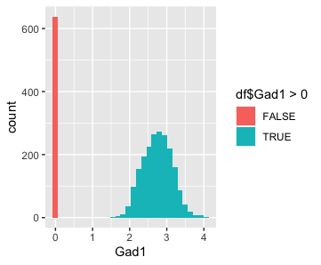
I am visualizing quantitative data of the expression level of the Gad1 gene, as well as ordinal data of the detection of the Gad1 gene, across spots in the Visium dataset.

I am using the geometric primitive of areas to encode this information.

I am using the visual channel of position on the x axis to encode the Gad1 expression level in the form of the counts-per-million normalized gene expression level that is log10 transformed with a pseudocount of 1.

I am using the visual channel of position on the y axis to encode the frequency of spots that express Gad1 at different magnitudes.

I am also using the visual channel of hue to encode the ordinal data to distinguish between spots that have no detected expression of Gad1 versus spots that have some detected expression of Gad1.

My explanatory data visualization seeks to make more salient how there are two populations of spots in this data: one that have some detected expression of Gad1 and one that does not. I am using the Gestalt principle of similarity via color to emphasize the two different groups of spots.

data <- read.csv('~/Desktop/class/genomic-data-visualization/data/Visium_Cortex_varnorm.csv.gz')
gexp <- data[, 4:ncol(data)]
rownames(gexp) <- data[,1]

# CPM normalize
numgenes <- rowSums(gexp)
normgexp <- gexp/rowSums(gexp)*1e6

# plot
library(ggplot2) 
df <- data.frame(log10(normgexp[, c('Gad1', 'Slc32a1')]+1))
ggplot(data = df,
    mapping = aes(x = Gad1)) +
geom_histogram(mapping = aes(fill = df$Gad1 > 0))