Spatial Distribution of Microglia, Determined Using CX3CR1 Expression as a Proxy

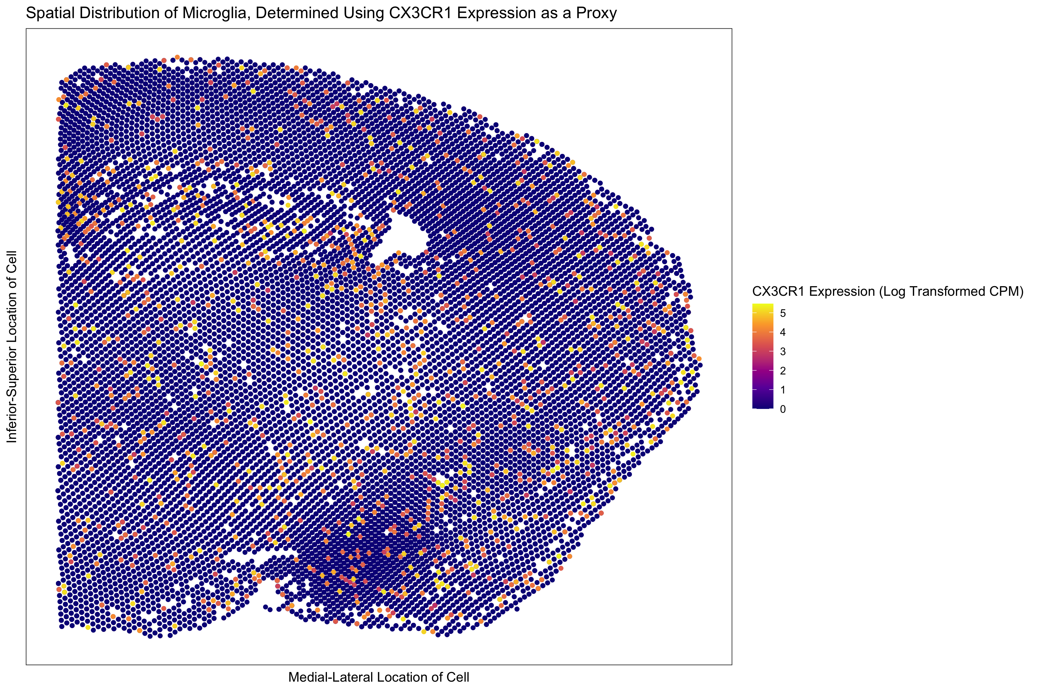
For homework 1, I chose to visualize quantitative data regarding the levels of expression of CX3CR1 (a marker whose expression I am using as a proxy for the identification of microglia) across the mouse brain from which the MERFISH dataset was derived.

I used the geometric primitive of points to represent single cells within our MERFISH dataset.

I used the visual channel of position along the x and y axes to encode the respective positions of cells across the mouse brain. In addition, I used the visual channel of color, specifically hue, to encode the level of CX3CR1 expression on a cell-by-cell basis. The expression of CX3CR1 was determined by performing a log10 transformation on the CX3CR1 counts per million (normalized to total transcripts in the cell) for each cell in the data set. A pseudocount of 1 was added to all CPM values to account for cells that do not express CX3CR1 in any capacity.

The overall goal of this data manipulation is to make more salient the claim that microglia are broadly distributed across the brain, perhaps because they play a major role in protecting neurons from non-self pathogens. To this end, I used the Gestalt principle of similarity by color. The microglia (cells that express CX3CR1 to varying extents) are a non-blue hue, while all other cell types—which do not express the microglia-specific CX3CR1 marker—are blue. As a result, it is very simple to identify microglia from other cells in our data visualization and ultimately observe that the spatial distribution of microglia is relatively homogenous across the brain. Furthermore, the color gradient I employed to encode the level of CX3CR1 expression helps to make the cells that do express CX3CR1 (i.e., microglia) stand out from cells that do not: the former are typically yellow, orange, or red, while the latter are invariably blue in color.

#Goal: Visualize the localization of microglia in the brain, using Cx3cr1 expression as a proxy
data <- read.csv("/Users/ares2081/Desktop/MERFISH_Slice2Replicate2_halfcortex.csv")
pos <- data[, c('x', 'y')]
rownames(pos) <- data[,1]
gexp <- data[, 4:ncol(data)]
rownames(gexp) <- data[,1]
#Check we can find microglia-specific gene in gexp
c('Cx3cr1') %in% colnames(data)
# CPM normalize
numgenes <- rowSums(gexp)
normgexp <- gexp/rowSums(gexp)*1e6
#Getting a sense of the number of Cx3cr1 RNAs per cell (logscale)
log10(normgexp[, 'Cx3cr1']+1)
#Appears to be between 0 to 100000
#Visualizing Cx3cr1 (microglia marker)
library(ggplot2)
#Using a pseudocount of 1 to account for cells that don't express Cx3cr1
df <- data.frame(x = pos[,1],
                 y = pos[,2],
                 gene = log10(normgexp[, "Cx3cr1"]+1))
#Implementing scale_color_gradient function to create unique expression scale 
#Based on code sourced from https://ggplot2.tidyverse.org/reference/ and https://ggplot2-book.org/scale-colour.html
#Plot editing was done based on code from https://rpubs.com/Mentors_Ubiqum/ggplot_remove_elements
install.packages('scico')#color gradients
ggplot(data = df,
       mapping = aes(x = x, y = y)) +
  geom_point(mapping = aes(col=gene), size=1.25) + 
  ggtitle("Spatial Distribution of Microglia, Determined Using CX3CR1 Expression as a Proxy") +
  labs(x = "Medial-Lateral Location of Cell", y = "Inferior-Superior Location of Cell", 
       color = "CX3CR1 Expression (Log Transformed CPM)") + scale_color_viridis_c(option = "plasma") +
  theme_bw() + theme(panel.grid.major = element_blank(), panel.grid.minor = element_blank(), 
                     axis.ticks.x=element_blank(), 
                     axis.text.x=element_blank(), axis.ticks.y=element_blank(),
                     axis.text.y=element_blank())
#Save plot as png
ggsave("saichandanreddy_hw1.png", plot=last_plot(), path="/Users/ares2081/Desktop/genomic-data-visualization-main/homework/hw1",
       width = 30, height = 20, units = 'cm')