Spatial Distribution of MERFISH RNA counts

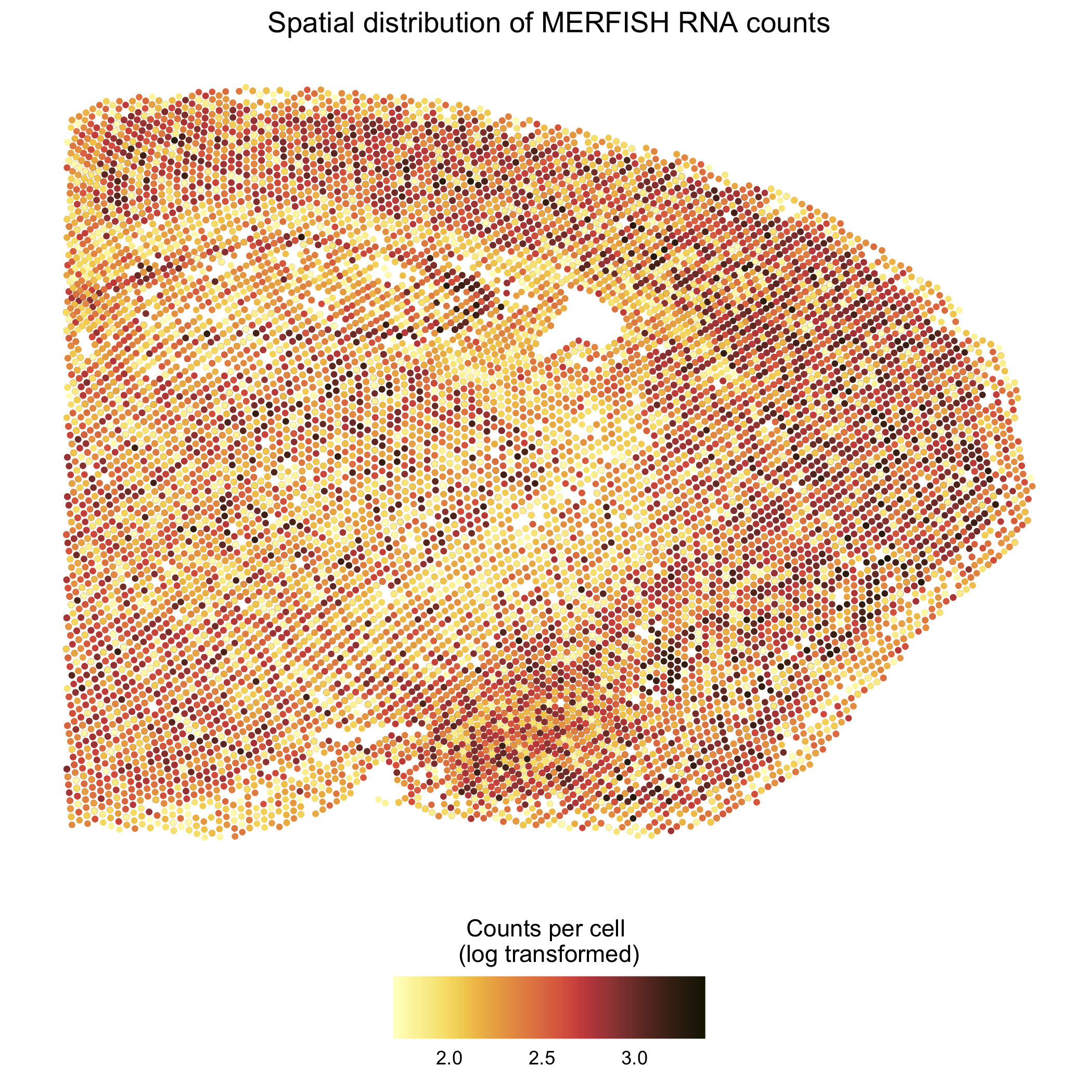
I am visualizing the relationship between the position of cells in the MERFISH dataset (quantitative) and the total RNA counts per cell (quantitative).

Here, the geometric primitive of points is used to represent cells, and the visual channel of position is used to encode cell position in the X and Y dimensions.

Finally, the visual channel of color is used to encode the total RNA counts per cell (log10 transformed with a pseudocount of 1).

In this data visualization, I try to make salient that the spatial distribution of RNA counts is not homogenous across the tissue and different regions of the brain may have more/less RNA expression.

library(ggplot2)
library(RSpectra)
library(colorBlindness)
library(scico)

### LOAD DATA ### 
data.dir <-  "/Users/lylaatta/Documents/GitHub/genomic-data-visualization/data/"
path.merfish <- paste0(data.dir,"MERFISH_Slice2Replicate2_halfcortex.csv.gz")
data.merfish <- read.csv(path.merfish, row.names = 1)

pos.merfish <- data.merfish[,c("x","y")]
counts.merfish <- data.merfish[,-c(1,2)]

merfish.total.counts <- log10(rowSums(counts.merfish)+1) #total counts per cell 
merfish.gene.counts <- log10(rowSums(counts.merfish>0)+1) #number of detected genes per cell 
df <- data.frame(cbind(pos.merfish, merfish.total.counts, merfish.gene.counts))
# head(df)

#lyla's theme: plot aesthetic settings that can be reused in multiple figures 
my.theme <- theme_classic() + theme(plot.title = element_text(hjust = 0.5), 
                                    axis.line=element_blank(),
                                    axis.title.x=element_blank(),
                                    axis.text.x=element_blank(),
                                    axis.ticks.x=element_blank(),
                                    axis.title.y=element_blank(),
                                    axis.text.y=element_blank(),
                                    axis.ticks.y=element_blank(),
                                    legend.position = "bottom",
                                    # panel.border = element_rect(color = "black", fill=NA)
)

ggplot(data = df, mapping = aes(x = x, y = y)) + 
  geom_point(mapping = aes(color = merfish.total.counts), size = 0.75) +
  scico::scale_color_scico(palette = "lajolla", #change color to make differences more clear, see: https://ggplot2-book.org/scale-colour.html
                           #limits = c(1,4), breaks = c(1,2,3,4), 
                           guide = guide_colorbar(direction = "horizontal", barheight = 2, barwidth = 10,
                                                  title.position = "top", title.hjust = 0.5, 
                                                  label.position = "bottom", ticks = FALSE)) +
  ggtitle("Spatial distribution of MERFISH RNA counts") + 
  xlab("X") + ylab("Y") + 
  labs(color='Counts per cell \n(log transformed)') +
  my.theme

#check that colors are colorblind friendly 
# colorBlindness::displayAllColors(scico(6, palette = "lajolla"))

#save as png 
ggsave("merfish_counts_space.png")