Identifying Dopaminergic Neurons Using the Expression of Robust Marker Th in a Spatially Resolved Manner

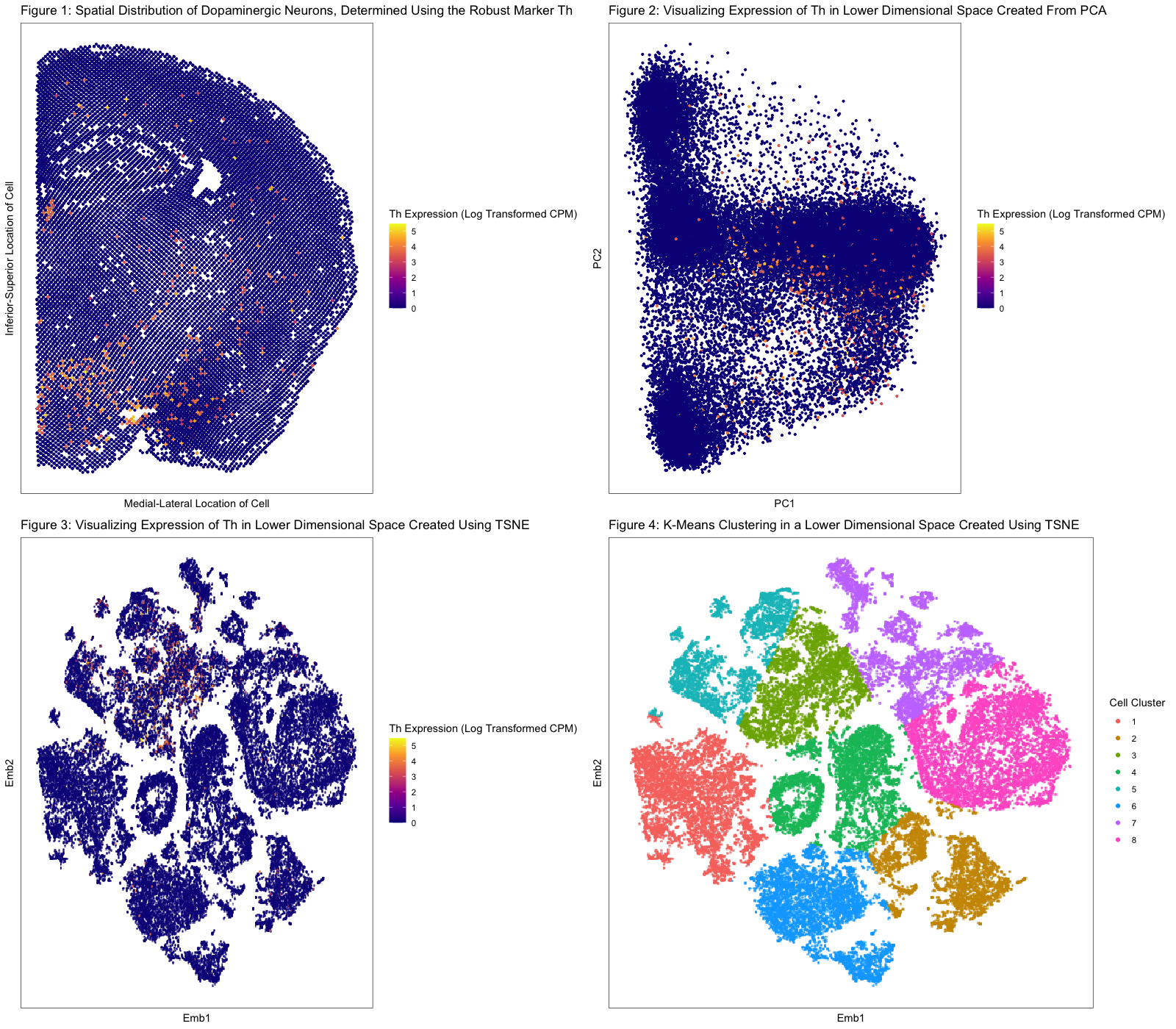
In Figure 1, I chose to visualize quantitative data regarding the levels of expression of Th (a marker whose expression I am using as a proxy for the identification of dopaminergic neurons) across the mouse brain from which the MERFISH dataset was derived. I used the geometric primitive of points to represent single cells within our MERFISH dataset. I used the visual channel of position along the x and y axes to encode the respective positions of cells across the mouse brain. In addition, I used the visual channel of color, specifically hue, to encode the level of Th expression on a cell-by-cell basis. The expression of Th was determined by performing a log10 transformation on the Th counts per million (normalized to total transcripts in the cell) for each cell in the data set. A pseudocount of 1 was added to all CPM values to account for cells that do not express Th in any capacity. Clearly, from this data visualization, we make more salient the point that within the mouse brain, the limbic system (medial/inferior region of our diagram) is incredibly enriched for expression of Th, suggesting this is where we will find our dopaminergic neurons clustered predominantly. Note, cells that expressed Th are grouped by the Gestalt principle of color (i.e., they will have a non-blue hue).
In Figure 2, I performed PCA on quantitative gene expression data from the MERFISH dataset to generate a lower dimensional space from principal components 1 and 2. Again, I used the geometric primitive of points to represent single cells within our MERFISH dataset. I used the visual channel of position along the x and y axes to encode the respective positions of cells in this lower dimensional space. Furthermore, I used the visual channel of color, specifically hue, to encode the level of Th expression (in normalized CPM) for each cell. The purpose of this data manipulation is to put forth the argument that it is difficult to visualize cell clustering by type (e.g., dopaminergic, glutaminergic, etc.) in a reduced dimensional space created from PCs 1 and 2. We see that cells that express Th, which are yellow, orange, or red, are rather spread out. This finding is easily seen by a viewer due to the Gestalt principle of grouping by similarity in color: when you group the Th- (blue) cells by color, you see there are numerous random insertions of Th+ cells, suggesting Th+ cells do not cluster well in this space. To sum, there is a need for non-linear dimensional reduction.
In Figure 3, I performed TSNE (non-linear dimensional reduction) on the PCA-derived space described in the previous paragraph, which in turn is derived from quantitative gene expression data. I used the geometric primitive of points to represent single cells within our MERFISH dataset. I also utilized the visual channel of position along the x and y axes to encode the respective positions of cells in this lower dimensional space and the channel of color, specifically hue, to encode the level of Th expression (in normalized CPM). Ultimately, the purpose of this data visualization is to show that cells form distinct groupings in the embedded space. This point is made poignantly given that cells, as indicated by points, can be grouped according to the Gestalt principle of grouping by proximity. Furthermore, when looking at Th expression in this reduced dimensional space, there appears to be a cluster of cells—identified readily using the Gestalt principle of grouping by similarity in color—that strongly expresses this marker for dopaminergic neurons.
In Figure 4, I performed K-means clustering on the embedded space derived using TSNE. The geometric primitive of points was used to represent cells in the reduced dimensional space. Again, the visual channel of position along the x and y axes represents the respective positions of cells in this lower dimensional space. The channel of color, specifically hue, was used to encode the cell clusters generated using K-means clustering. The purpose of this figure is to demonstrate that there are specific cell-clusters in our data set, and this point is strengthened by the Gestalt principle of grouping by similarity in color.
After generating these cell clusters, I compared the cluster that looked to have a high Th expression to the rest of the data set and found that Th gene expression was upregulated significantly (p-value from t-test: 9.876837e-155, p-value from Wilcoxon-test: <2.2e-16). Furthermore, using a “for loop” to search for other differentially upregulated genes in the Th+ cell cluster, I found that the family of genes encoding 5-HT receptors (mainly, Htr2c, Htr4, Htr5a, and Htr7) were also overexpressed. This is an important finding because dopaminergic neurons have been shown to highly express these genes (Bubar & Cunningham, 2007). Overall, there is strong support that Th is a robust marker for identification of dopaminergic neurons in the mouse brain.
#Goal: Visualizing the Location of Dopaminergic Neurons Using the Expression of Robust Marker Th
data <- read.csv("/Users/ares2081/Desktop/MERFISH_Slice2Replicate2_halfcortex.csv")
pos <- data[, c('x', 'y')]
rownames(pos) <- data[,1]
gexp <- data[, 4:ncol(data)]
rownames(gexp) <- data[,1]
#Check we can find Dopaminergic-neuron-specific gene Th (which codes for tyrosine hydroxylase) in gexp
c('Th') %in% colnames(data)
#CPM normalize
numgenes <- rowSums(gexp)
normgexp <- gexp/rowSums(gexp)*1e6
#Getting a sense of the number of Th RNAs per cell (logscale)
log10(normgexp[, 'Th']+1)
#Appears to be between 0 and 5
#Spatial Visualization of Th
library(ggplot2)
df1 <- data.frame(x = pos[,1],
                 y = pos[,2],
                 gene = log10(normgexp[, "Th"]+1))
p1 <- ggplot(data = df,
             mapping = aes(x = x, y = y)) +
  geom_point(mapping = aes(col=gene), size=0.75) +
  ggtitle("Figure 1: Spatial Distribution of Dopaminergic Neurons, Determined Using the Robust Marker Th") +
  labs(x = "Medial-Lateral Location of Cell", y = "Inferior-Superior Location of Cell",
       color = "Th Expression (Log Transformed CPM)") + scale_color_viridis_c(option = "plasma") +
  theme_bw() + theme(panel.grid.major = element_blank(), panel.grid.minor = element_blank(),
                     axis.ticks.x=element_blank(),
                     axis.text.x=element_blank(), axis.ticks.y=element_blank(),
                     axis.text.y=element_blank())
p1
#PCA (linear dimension reduction)
mat <- log10(normgexp+1)
pcs <- prcomp(mat)
names(pcs)
dim(pcs$x)
plot(pcs$sdev[1:30], type='l')
#It appears the first 15 PCs capture most of the standard deviation.
#Check if we can identify a cluster of Th+ cells (presumably dopaminergic neurons) by visualizing the data using PCs 1 and 2.
df2 <- data.frame(pc1 = pcs$x[,1],
                  pc2 = pcs$x[,2],
                  col = mat[, 'Th'])
p2 <- ggplot(data = df2,
       mapping = aes(x = pc1, y = pc2)) +
  geom_point(mapping = aes(col=col), size=0.75) +
  ggtitle("Figure 2: Visualizing Expression of Th in Lower Dimensional Space Created From PCA") +
  labs(x = "PC1", y = "PC2", color = "Th Expression (Log Transformed CPM)") +
  scale_color_viridis_c(option = "plasma") + theme_bw() + theme(panel.grid.major = element_blank(),
                                                                panel.grid.minor = element_blank(), axis.ticks.x=element_blank(),
                                                                axis.text.x=element_blank(), axis.ticks.y=element_blank(),axis.text.y=element_blank())
p2
#It is fairly difficult to identify a distinctive cluster of Th+ cells in PC-space.
#Plotting the first 3 PCs, we see they don't truly capture all of the variation in our transcriptomic data.
df3 <- data.frame(pc1 = pcs$x[,1],
                 pc2 = pcs$x[,2],
                 col = pcs$x[,3])
p3 <- ggplot(data = df3,
       mapping = aes(x = pc1, y = pc2)) +
  geom_point(mapping = aes(col=col))
p3
#Consequently, let's apply a non-linear dimensional reduction to our PCs (TSNE).
library(Rtsne)
set.seed(0)
emb <- Rtsne(pcs$x[, 1:15], dims=2, perplexity = 30)$Y
rownames(emb) <- rownames(mat)
#Plot MERFISH data in reduced 2-dimensional space
plot(emb, pch=".")
#Assess expression of Th in lower dimensional space
df4 <- data.frame(x = emb[,1],
                 y = emb[,2],
                 col = mat[, 'Th'])
library(scattermore)
p4 <- ggplot(data = df4,
       mapping = aes(x = x, y = y)) +
  geom_scattermore(mapping = aes(col = col), pointsize=0.75) +
  ggtitle("Figure 3: Visualizing Expression of Th in Lower Dimensional Space Created Using TSNE") +
  labs(x = "Emb1", y = "Emb2", color = "Th Expression (Log Transformed CPM)") +
  scale_color_viridis_c(option = "plasma") + theme_bw() + theme(panel.grid.major = element_blank(),
                                                                panel.grid.minor = element_blank(), axis.ticks.x=element_blank(),
                                                                axis.text.x=element_blank(), axis.ticks.y=element_blank(),axis.text.y=element_blank())
p4
#K-means clustering in embedding space
set.seed(0)
com <- kmeans(emb, centers=8)
#Number of centers selected on the basis of number of groups seen in lower dimensional spatial visualization
df5 <- data.frame(x = emb[,1],
                 y = emb[,2],
                 col = as.factor(com$cluster))
p5 <- ggplot(data = df5,
             mapping = aes(x = x, y = y)) +
  geom_scattermore(mapping = aes(col = col), pointsize=0.75) +
  ggtitle("Figure 4: K-Means Clustering in a Lower Dimensional Space Created Using TSNE") +
  labs(x = "Emb1", y = "Emb2", color = "Cell Cluster") + scale_fill_discrete() + theme_bw() + theme(panel.grid.major = element_blank(),
                                                                                       panel.grid.minor = element_blank(), axis.ticks.x=element_blank(),
                                                                                       axis.text.x=element_blank(), axis.ticks.y=element_blank(),axis.text.y=element_blank())
p5
#By comparing p3 with p2, we can see that cluster 3 likely houses our Th+ dopaminergic cells.
#To confirm this we can see if Th is differentially upregulated in cluster 3 compared to other clusters using a T-test.
iii <- com$cluster == 3
g <- 'Th'
x = t.test(mat[iii, g], mat[!iii, g], alternative='greater')
x$p.value
#p-value = 9.876837e-155
#The t-test indicated that Th was expressed to a substantially higher extent in cluster 3 compared to other clusters.
#Due to the possibility our data isn't entirely normal, let's also run a Wilcoxon test to confirm if Th is differentially upregulated in cluster 7.
y = wilcox.test(mat[iii, g], mat[!iii, g], alternative='greater')
y$p.value
#p-value<2.2e-16
#The Wilcoxon test indicated that Th was differentially upregulated in cluster 3 compared to other clusters.
#Conclusion: cluster 3 is enriched for Th expression.
#Overall, the t-test and Wilcoxon test both indicate that our cluster 3 likely corresponds to Dopaminergic neurons.
#Next, I would like to see what other genes are differentially upregulated in cluster 3, using the Wilcoxon test in combination with a "for loop."
diff <- sapply(colnames(mat), function(g) {x = wilcox.test(mat[vii, g], mat[!vii, g], alternative='greater')
  return(x$p.value)})
#Since we are running the Wilcoxon test iteratively, we will need to apply a Bonferroni correction to account for false significant results.
p.adjust(diff)
sorted_diff <- sort(-log10(p.adjust(diff)), decreasing=TRUE)
sorted_diff[1:10]
#The top-10 most differentially expressed genes (in terms of expression) are given below.
#Htr2c   Htr4  Htr5a   Htr7 Adgra1 Adgrb3 Adgrl3 Adra1a  Ackr1 Celsr3
#Htr2c   Htr4  Htr5a   Htr7 are a group of genes that encode 5-HT (hydroxytryptamine) receptors, which are frequently expressed by dopaminergic neurons (Bubar & Cunningham, 2007).
#This finding supports our claim that Th is a valid marker for identification of dopaminergic neurons in a spatially resolved manner.
#Overall, we were able to use PCA, TSNE, K-means clustering, and differential gene expression analysis to show that Th,...
#...the gene encoding tyrosine hydroxylase, can be used to identify dopaminergic neurons in the mouse brain.
#Multi-panel generation
library(gridExtra)
grid.arrange(p1, p2, p4, p5, ncol=2)