Exploration of GFAP expression in Kmeans Clustering of MERFISH data

I am visualizing quantitative data of the expression level after TSNE embedding and kmeans clustering based on that in the MERFISH dataset.

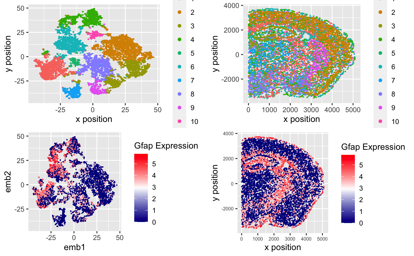
In these 4 plots, I’m using the geometric primitive of points to encode different cells in this dataset.

In the top-left plot, I’m using the visual channel of hues to encode different clusters formed by kmeans method and position of (x,y) coordinates to encode the similarity between cells.

In the top-right plot, I’m using the visual channel of hues to encode different clusters formed by kmeans method and position of (x,y) coordinates to encode the physical position of cells in this cortex biopsy.

In the bottom-left plot, I’m using the visual channel of hues to encode GFAP expression level and position of (x,y) coordinates to encode the similarity between cells after kmeans clustering.

In the bottom-right plot, I’m using the visual channel of hues to encode GFAP expression level and position of (x,y) coordinates to encode the physical position of cells in this biopsy.

From the top 2 plots, I want to confirm that clusters in kmeans clustering do encode the similarity between cells. We can double check that these clusters of cells form real structures in the biopsy.

In the bottom 2 plots, I want to do some exploration on the GFAP expression in this dataset. I noticed that from the bottom-left plot, GFAP is selectively upregulated in cluster 6 and 10, also we see this specific expression pattern in the position plot on bottom-right, which suggests that GFAP may be a marker gene for some type of cells in the cortex.

Here I’m using the Gestalt Principle of Proximity to stress the similarity between cells in Top plots while using Gestalt Principle of Similarity in hues to encode the expression level groups in bottom plots.

library(ggplot2)
library(scattermore)
data<-read.csv("MERFISH_Slice2Replicate2_halfcortex.csv.gz")
pos <- data[, c('x', 'y')]
rownames(pos) <- data[,1]
gexp <- data[, 4:ncol(data)]
rownames(gexp) <- data[,1]

data_sub <- sample(rownames(pos), 10000) #down sample data to 10000 cells

pos <- pos[data_sub,]
gexp <- gexp[data_sub, ]

#CPM normalization
numgenes <- rowSums(gexp)
normgexp <- gexp/numgenes*1e6
#matrix of gene expression
mat <- log10(normgexp + 1)

# PCA and Tsne analysis
pcs <- prcomp(mat)
plot(pcs$sdev[1:30], type="l")
library(Rtsne)
set.seed(0)
emb <- Rtsne(pcs$x[,1:10], dims=2, perplexity=30)$Y

# do k-means clustering based on gene expression levels
set.seed(0)
clus<- kmeans(mat,centers = 10)
df1 <- data.frame(x = emb[,1],
                 y = emb[,2],
                 col = as.factor(clus$cluster)) 
p1 <- ggplot(data = df1,
            mapping = aes(x = x, y = y)) +
  geom_scattermore(mapping = aes(col = col), 
                   pointsize=3)
plot1<-p1+ labs(x = "x position" , y = "y position")


df2 <- data.frame(x = pos[,1],
                 y = pos[,2],
                 Clusters = as.factor(clus$cluster))
p2<- ggplot(data = df2,
               mapping=aes( x=x, y=y))+
  geom_scattermore(mapping = aes( col= Clusters),pointsize = 3)
plot2<- p2+ labs(x = "x position" , y = "y position")

tgene <- 'Gfap'
df3 <- data.frame(x = emb[,1],
                 y = emb[,2],
                 Gfap_expression = mat[, tgene])
plot3 <- ggplot(data = df3,
            mapping = aes(x = x, y = y)) +
  geom_scattermore(mapping = aes(col = Gfap_expression), 
                   pointsize = 3)+
  scale_color_gradientn("Gfap Expression", 
                        colours = colorRampPalette(
                          c("darkblue", "white", "red"))(50)
  ) + labs(x = "emb1" , y = "emb2")
plot3
df4 <- data.frame(x = pos[,1],
                 y = pos[,2],
                 Gfap_expression = mat[, tgene])
plot4 <- ggplot(data = df4,
            mapping = aes(x = x, y = y), cex.axis=0.8) +
  geom_scattermore(mapping = aes(col = Gfap_expression), 
                   pointsize=3)+
  scale_color_gradientn("Gfap Expression", 
                        colours = colorRampPalette(
                          c("darkblue", "white", "red"))(50)
  )+ labs(x = "x position" , y = "y position") + theme(axis.text.x = element_text( size=6),axis.text.y = element_text(size=6))

plot4
grid.arrange(plot1, plot2, plot3, plot4, ncol=2)