identify and visualize the spatial distribution of Mature Oligodendrocytes

My reasoning for why this specific group of cells stands for potentially mature oligodendrocytes:

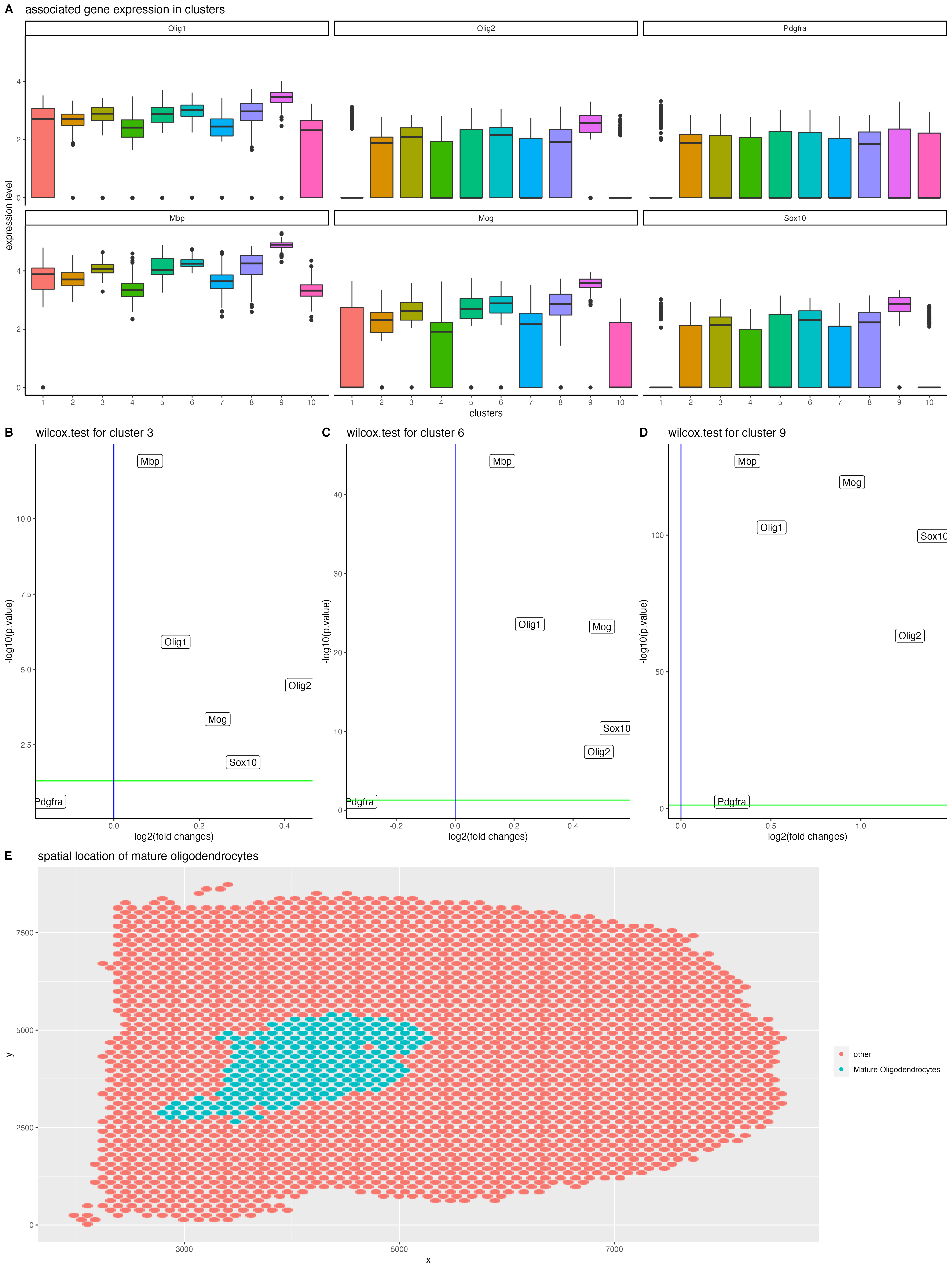
Figure1: First I did kmeans clustering based on gene expressions and get 10 clusters. Then I sorted out the valuable genes for detecting mature oligodendrocytes, namely “target_genes”. Based on that, I plot a boxplot to show target genes’ expression levels among different clusters, as is shown in figure1. Look into figure1, I sorted out 3 possible clusters that could possibly represent mature oligodendrocytes. They are cluster 3, 6 and 9, sharing the same expression pattern of “High Olig1 and Olig2 expression” & “Relatively low Pdgfra expression” & “High Mbp, Mog and Sox10 expression”.

Figure2: To be numerate and convince myself statistically, I did wilcox.test for all target genes among clusters, computed p.values and fold changes and summarized them within a volcano plot as shown in figure2. For better visualization, I drew a green line where p.value is equal to 0.05, and the blue line indicates where the fold.change is equal to 1. Thus, from Figure2, I convince myself that cluster9 may not be mature oligodendrocytes since its fold change for pdgfra is over 1. And to our knowledge, mature oligodendrocytes do not express pdgfra. For the same reason, I believe that cluster6 has a higher probability of being mature oligodendrocytes since its p.value for pdgfra is close to the significant level while fold change is way less than 1, which indicates its expression of pdgfra is significantly less.

Figure3: To visualize spatial distribution of cluster6, which is my potential mature oligodendrocytes, I did a plot based on spatial positions of detecting points and specially lighted up cluster6 with blue dots.

#load packages
library(tidyverse)
library(ggplot2)
library(scattermore)
library(reshape2)
require(devtools)
library(highcharter)
library(magrittr)
library(gridExtra)

#read in data, recode variables and spot valuable genes
data<-read.csv("Visium_Cortex_varnorm.csv.gz")
gexp<- data[,4:ncol(data)]
pos<- data[,2:3]
numgenes <- rowSums(gexp)
normgexp <- gexp/numgenes*1e6
mat <- log10(normgexp+1)
rownames(mat)<-data[,1]
#check if marker genes selected are in this dataset
'Olig1' %in% colnames(data)
'Olig2' %in% colnames(data)
'Olig3' %in% colnames(data)
'Pdgfra' %in% colnames(data)
'Osp' %in% colnames(data)
'Mbp' %in% colnames(data)
'Mog' %in% colnames(data)
'Sox10' %in% colnames(data)
target_genes<-c("Olig1","Olig2","Pdgfra","Mbp","Mog","Sox10")

#kmeans clustering
set.seed(0)
com <- kmeans(mat, centers=10)

#target gene expression among clusters
df <- reshape2::melt(
  data.frame(id=rownames(mat),mat[, target_genes], 
             clusters=as.factor(com$cluster)))
df_pos<-cbind(pos[,1:2],df[,2])
p1 <- ggplot(data = df,
       mapping = aes(x=clusters, y=value, fill=clusters)) + 
  labs(y="expression level" , x="clusters", title = "Figure1: associated gene expression in clusters")+
  geom_boxplot(show.legend = FALSE) + 
  theme_classic() + 
  facet_wrap( ~ variable)

#wilcox.test for selected clusters
gexp<- mat[,target_genes]
df_pos<- data.frame(x=pos[,1],y=pos[,2],
                cluster = com$cluster)
m<- cbind(df_pos[,3],gexp[,1:6])
cluster3 <- com$cluster==3
cluster6 <- com$cluster==6
cluster9 <- com$cluster==9

for(i in 1:5) {
  print(i)
}

x = sapply(1:5, function(i) {
  print(i)
  return(i)
})

pvs6 <- sapply(colnames(gexp), function(g) {
  x = wilcox.test(mat[cluster6, g], mat[!cluster6, g], 
      alternative='two.sided')
  return(x$p.value)
})

fcs6 <- sapply(colnames(gexp), function(g) {
  x = mean(mat[cluster6, g])/mean(mat[!cluster6, g])
  return(x)
})

df6 <- data.frame(name = colnames(gexp), 
                 pvs = -log10(pvs6), 
                 fcs = log2(fcs6))
p6 <- ggplot(df6, mapping = aes(x=fcs, y=pvs)) + 
  geom_point() + geom_label(mapping = aes(label = name)) +
  theme_classic()+labs( title='wilcox.test for cluster 6', x ='log2(fold changes)', y='-log10(p.value)') + 
  geom_abline(intercept= -log10(0.05),slope= 0, col="green") +
  geom_vline(xintercept = log2(1),col="blue")


pvs3 <- sapply(colnames(gexp), function(g) {
  x = wilcox.test(mat[cluster3, g], mat[!cluster3, g], 
      alternative='two.sided')
  return(x$p.value)
})

fcs3 <- sapply(colnames(gexp), function(g) {
  x = mean(mat[cluster3, g])/mean(mat[!cluster3, g])
  return(x)
})

df3 <- data.frame(name = colnames(gexp), 
                 pvs = -log10(pvs3), 
                 fcs = log2(fcs3))
p3 <- ggplot(df3, mapping = aes(x=fcs, y=pvs)) + 
  geom_point() +
  geom_label(mapping = aes(label = name)) + theme_classic()+labs( title='wilcox.test for cluster 3', x ='log2(fold changes)', y='-log10(p.value)')+ geom_abline(intercept= -log10(0.05),slope= 0, col="green")+
  geom_abline(intercept= -log10(0.05),slope= 0, col="green") +
  geom_vline(xintercept = log2(1),col="blue")


pvs9 <- sapply(colnames(gexp), function(g) {
  x = wilcox.test(mat[cluster9, g], mat[!cluster9, g], 
      alternative='two.sided')
  return(x$p.value)
})
fcs9 <- sapply(colnames(gexp), function(g) {
  x = mean(mat[cluster9, g])/mean(mat[!cluster9, g])
  return(x)
})
df9 <- data.frame(name = colnames(gexp), 
                 pvs = -log10(pvs9), 
                 fcs = log2(fcs9))
p9 <- ggplot(df9, mapping = aes(x=fcs, y=pvs)) + 
  geom_point() +
  geom_label(mapping = aes(label = name)) + 
  theme_classic()+
  labs( title='wilcox.test for cluster 9', x ='log2(fold changes)', y='-log10(p.value)') +
  geom_abline(intercept= -log10(0.05),slope= 0, col="green") +
  geom_vline(xintercept = log2(1),col="blue")

p2<- grid.arrange(p3,p6,p9, ncol=3)

#spatial locations and joined plots display
locate <-  ggplot(data = df_pos,
            mapping = aes(x = x, y = y),show.legend=FALSE) +
  geom_scattermore(mapping = aes(col = cluster6), 
                   pointsize=3) +
  labs(title = "Figure2: locate mature oligodendrocyte") +
  scale_colour_hue("",breaks=c("FALSE","TRUE"),labels=c("other","Mature Oligodendrocytes"))



row_1<- plot_grid( p1,locate,ncol=1, nrow=1)
row_2<- plot_grid( p3, p6, p9,ncol=3, nrow=1, rel_widths = c(1,1,1))
row_3<- plot_grid( locate,ncol=1, nrow=1)

plot_grid(row_1,row_2,row_3,nrow = 3)

ggsave("Stella Li.png",width=15,height =20 )