Identifying Mature Oligodendrocytes Using the Canonical Marker Olig1

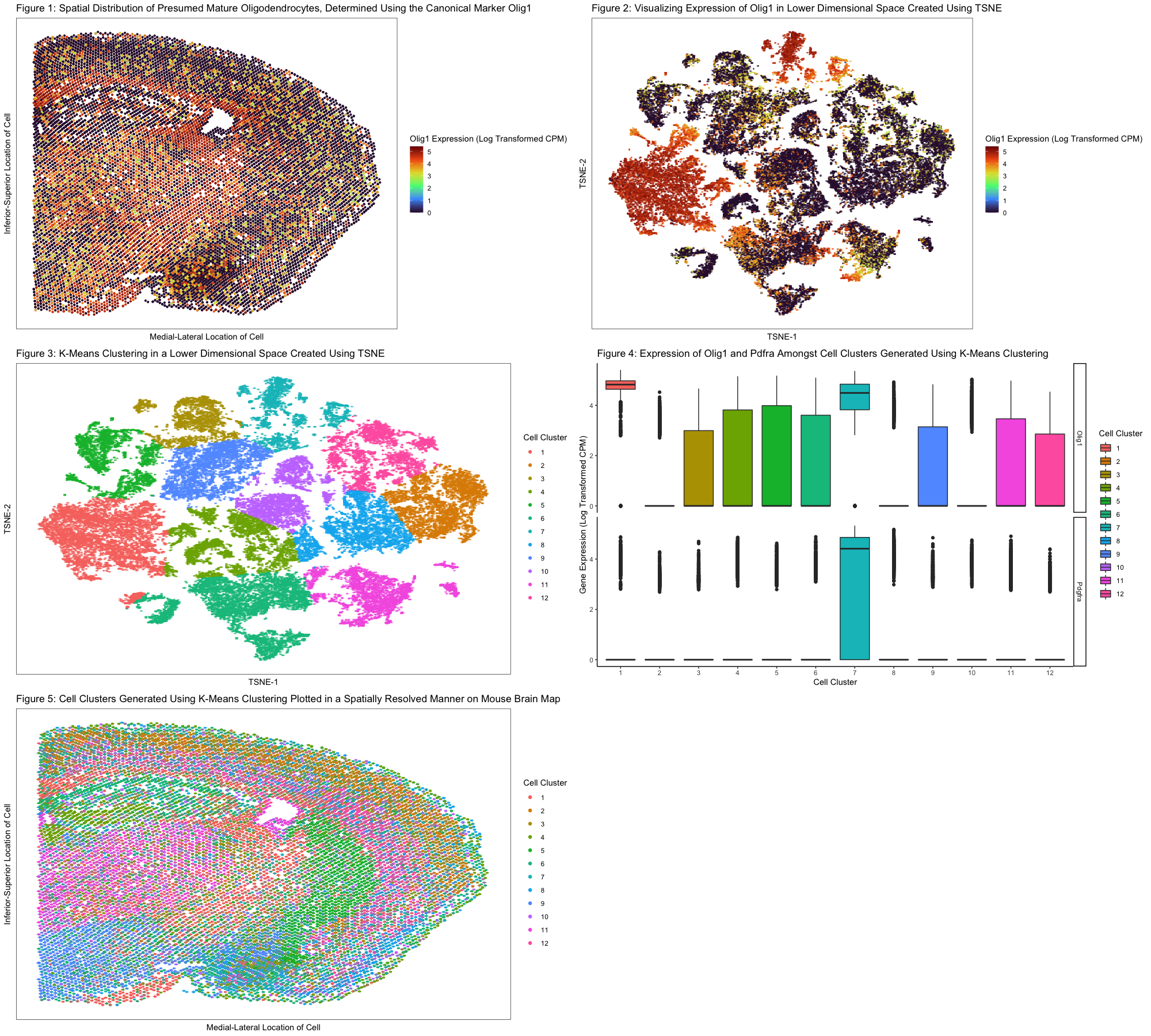
In Figure 1, I chose to visualize quantitative data regarding the levels of expression of Olig1 (a canonical marker endogenous to mature oligodendrocytes as well as oligodendrocyte precursor cells) across the mouse brain from which the MERFISH dataset was derived. I used the geometric primitive of points to represent single cells within our MERFISH dataset. I used the visual channel of position along the x and y axes to encode the respective positions of cells across the mouse brain. In addition, I used the visual channel of color, specifically hue, to encode the level of Olig1 expression on a cell-by-cell basis. The expression of Olig1 was determined by performing a log10 transformation on the normalized Olig1 counts per million for each cell in the data set. A pseudocount of 1 was added to all CPM values to account for cells that do not express Olig1 in any capacity. Clearly, from this data visualization, we make more salient the point that oligodendrocytes are distributed across the brain, which is a logical finding given the pertinent role they play in myelinating the axons of all the neurons in the brain.
In Figure 2, I performed TSNE analysis (non-linear dimensional reduction) on principal components 1 through 20, creating a 2-dimentional space derived from PC-space. I used the geometric primitive of points to represent single cells within our MERFISH dataset. I also utilized the visual channel of position along the x and y axes to cluster cells based on transcriptional similarity. In this lower dimensional space and the channel of color, specifically hue, to encode the level of Olig1 expression (in normalized CPM). Ultimately, the purpose of this data visualization is to show that cells form distinct groupings in the embedded space. This point is made poignantly given that cells, as indicated by points, can be grouped according to the Gestalt principle of grouping by proximity. Furthermore, when looking at Olig1 expression in this reduced dimensional space, there appears to be two cluster of cells—identified readily using the Gestalt principle of grouping by similarity in color—that strongly express this marker for mature oligodendrocytes.
In Figure 3, I performed K-means clustering on the embedded space derived using TSNE. The geometric primitive of points was used to represent cells in the reduced dimensional space. Again, the visual channel of position along the x and y axes represents the grouping of cells based on transcriptional similarity. The channel of color, specifically hue, was used to encode the cell clusters generated using K-means clustering. The purpose of this figure is to demonstrate that there are specific cell-clusters in our data set, and this point is strengthened by the Gestalt principle of grouping by similarity in color.
After generating these cell clusters, I noticed that there were two clusters that had high expression of Olig1: clusters 1 and 7. I compared each of the clusters to the rest of the data set and found that Olig1 gene expression was upregulated significantly (p-value from t-test: <2.2e-16 and p-value from Wilcoxon-test: <2.2e-16, for both clusters). However, due to the high likelihood one of these clusters corresponded to oligodendrocyte precursor cells (OPCs), which express Olig1 like mature oligodendrocytes, I checked both clusters for upregulation of Pdgfra (a marker specific to OPCs). Cluster 1 did not show upregulation of Pdgfra, but cluster 7 did, leading me to conclude that cluster 7 corresponds to OPCs. This information is shown in the box plots depicted in figure 4. In Figure 5, we projected the cell clusters derived from k-means clustering onto the original mouse brain map to identify the spatial location of mature oligodendrocytes. Again, the same color scheme as in figure 4 was used to represent specific clusters of cells. It appears mature oligodendrocytes, red in color—i.e., color corresponding to cluster 1, are spread out across the mouse brain. This point is made more salient due to the use of Gestalt principle of grouping by similarity in color.
Finally, using a “for loop” to search for other differentially expressed genes in the mature oligodendrocyte cluster (i.e., cluster 1), I found that Gpr62 was also overexpressed among cells in cluster 1. Like Olig1, Gpr62 is a robust marker specific to mature oligodendrocytes (Hay et al., 2021), further supporting our belief that we have successfully identified mature oligodendrocytes in our dataset.
References:
-
Hay, C.M., Jackson, S., Mitew, S. et al. The oligodendrocyte-enriched orphan G protein-coupled receptor Gpr62 is dispensable for central nervous system myelination. Neural Dev 16, 6 (2021). https://doi.org/10.1186/s13064-021-00156-y
-
Fan, Jean (2022, February 14). Genomic Data Visualization Classnotes 20220214. Johns Hopkins University.
#Goal: Show that Olig1 is an Appropriate Marker for Identification of Mature Oligodendrocytes
data <- read.csv("/Users/ares2081/Desktop/MERFISH_Slice2Replicate2_halfcortex.csv")
pos <- data[, c('x', 'y')]
rownames(pos) <- data[,1]
gexp <- data[, 4:ncol(data)]
rownames(gexp) <- data[,1]
#Check we can find Oligodendrocyte-specific gene Olig1 in gexp
c('Olig1') %in% colnames(data)
#CPM normalize
numgenes <- rowSums(gexp)
normgexp <- gexp/rowSums(gexp)*1e6
#Getting a sense of the number of Th RNAs per cell (logscale)
log10(normgexp[, 'Olig1']+1)
#Many cells express Olig1, with values ranging from 1-5 (log scale)


#Spatial Visualization of Olig1
library(ggplot2)
df1 <- data.frame(x = pos[,1],
                  y = pos[,2],
                  gene = log10(normgexp[, "Olig1"]+1))
p1 <- ggplot(data = df1,
             mapping = aes(x = x, y = y)) +
  geom_point(mapping = aes(col=gene), size=0.75) +
  ggtitle("Figure 1: Spatial Distribution of Presumed Mature Oligodendrocytes, Determined Using the Canonical Marker Olig1") +
  labs(x = "Medial-Lateral Location of Cell", y = "Inferior-Superior Location of Cell",
       color = "Olig1 Expression (Log Transformed CPM)") + scale_color_viridis_c(option = "turbo") +
  theme_bw() + theme(panel.grid.major = element_blank(), panel.grid.minor = element_blank(),
          axis.ticks.x=element_blank(),
          axis.text.x=element_blank(), axis.ticks.y=element_blank(),
          axis.text.y=element_blank())
p1
#It appears oligodendrocytes are distributed rather evenly across the brain, implying the major role they play in myelinating axons of all neurons.


#PCA (linear dimension reduction)
mat <- log10(normgexp+1)
pcs <- prcomp(mat)
names(pcs)
dim(pcs$x)
plot(pcs$sdev[1:30], type='l')
#It appears the first 20 PCs capture most of the standard deviation.
#Plotting the first 3 PCs, we see they don't truly capture all of the variation in our transcriptomic data.
df2 <- data.frame(pc1 = pcs$x[,1],
                  pc2 = pcs$x[,2],
                  col = pcs$x[,3])
p2 <- ggplot(data = df2,
             mapping = aes(x = pc1, y = pc2)) +
  geom_point(mapping = aes(col=col))
p2


#To rectify this short coming, we will be applying a non-linear dimensionality reduction.
library(Rtsne)
set.seed(0)
emb <- Rtsne(pcs$x[, 1:20], dims=2, perplexity = 30)$Y
rownames(emb) <- rownames(mat)
#Plot MERFISH data in reduced 2-dimensional space
plot(emb, pch=".")
#Depict expression of Olig1 in reduced dimensional space
df3 <- data.frame(x = emb[,1],
                  y = emb[,2],
                  col = mat[, 'Olig1'])
library(scattermore)
p3 <- ggplot(data = df3,
             mapping = aes(x = x, y = y)) +
  geom_scattermore(mapping = aes(col = col), pointsize=0.75) +
  ggtitle("Figure 2: Visualizing Expression of Olig1 in Lower Dimensional Space Created Using TSNE") +
  labs(x = "TSNE-1", y = "TSNE-2", color = "Olig1 Expression (Log Transformed CPM)") +
  scale_color_viridis_c(option = "turbo") + theme_bw() + theme(panel.grid.major = element_blank(),
       panel.grid.minor = element_blank(), axis.ticks.x=element_blank(),
       axis.text.x=element_blank(), axis.ticks.y=element_blank(),axis.text.y=element_blank())
p3


#K-means clustering in embedding space
set.seed(0)
com <- kmeans(emb, centers=12)
#Number of centers selected on the basis of number of groups seen in lower dimensional spatial visualization
df4 <- data.frame(x = emb[,1],
                  y = emb[,2],
                  col = as.factor(com$cluster))
p4 <- ggplot(data = df4,
             mapping = aes(x = x, y = y)) +
  geom_scattermore(mapping = aes(col = col), pointsize=0.75) +
  ggtitle("Figure 3: K-Means Clustering in a Lower Dimensional Space Created Using TSNE") +
  labs(x = "TSNE-1", y = "TSNE-2", color = "Cell Cluster") + theme_classic() + theme_bw() + theme(panel.grid.major = element_blank(),
      panel.grid.minor = element_blank(), axis.ticks.x=element_blank(),
      axis.text.x=element_blank(), axis.ticks.y=element_blank(),axis.text.y=element_blank())
p4
#By comparing p4 with p3, we can see that clusters 1 and 7 likely house our mature oligodendrocytes.


#To confirm this we can see if Olig1 is differentially upregulated in clusters 1 and 7 compared to other clusters using a T-test.
#Start with cluster 1
i <- com$cluster == 1
g <- 'Olig1'
x = t.test(mat[i, g], mat[!i, g], alternative='greater')
x$p.value
#p-value<2.2e-16
#The t-test indicated that Olig1 was expressed to a substantially higher extent in cluster 1 compared to other clusters.
#Due to the possibility our data isn't entirely normal, let's also run a Wilcoxon test to confirm if Olig1 is differentially upregulated in cluster 1.
y = wilcox.test(mat[i, g], mat[!i, g], alternative='greater')
y$p.value
#p-value<2.2e-16
#The Wilcoxon test indicated that Olig1 was differentially upregulated in cluster 1 compared to other clusters.
#Conclusion: cluster 1 is enriched for Th expression.
#Check cluster 7 for upregulation of Olig1
vii <- com$cluster == 7
g <- 'Olig1'
r = t.test(mat[vii, g], mat[!vii, g], alternative='greater')
r$p.value
#p-value<2.2e-16
#The t-test indicated that Olig1 was expressed to a substantially higher extent in cluster 7 compared to other clusters.
s = wilcox.test(mat[vii, g], mat[!vii, g], alternative='greater')
s$p.value
#p-value<2.2e-16
#The Wilcoxon test indicated that Olig1 was differentially upregulated in cluster 1 compared to other clusters.
#Question: Do both clusters 1 and 7 correspond to distinct population of mature oligodendrocytes or is only one of these clusters truly mature oligodendrocytes?
#Because oligodendrocyte progenitors also express Olig1, to see if one of our clusters corresponds to OPCs, we can see if there is an overexpression of Pdgfra (OPC marker).
#Check cluster 1 for high expression of Pdgfra
opc <- 'Pdgfra'
a = wilcox.test(mat[i, opc], mat[!i, opc], alternative='greater')
a$p.value
#p-value=1, thus cluster 1 does not have upregulated expression of Pdgfra and does not correspond to OPCs.
#Check cluster 7 for high expression of Pdgfra
b = wilcox.test(mat[vii, opc], mat[!vii, opc], alternative='greater')
b$p.value
#p-value<2.2e-16, thus cluster 7 does have differentially upregulated expression of Pdgfra and does correspond to OPCs.
#Representing the overall findings regarding Olig1 and Pdgfra expression in clusters derived from K-means clustering.
df5 <- reshape2::melt(data.frame(id=rownames(mat), mat[, c('Olig1', 'Pdgfra')], col=as.factor(com$cluster)))
p5 <- ggplot(data = df5, mapping = aes(x=col, y=value, fill=col)) + geom_boxplot() + theme_classic() + facet_grid(variable ~ .) +
  ggtitle("Figure 4: Expression of Olig1 and Pdfra Amongst Cell Clusters Generated Using K-Means Clustering") +
  labs(x = "Cell Cluster", y = "Gene Expression (Log Transformed CPM)", fill = "Cell Cluster")
p5

#Identifying other differentially unregulated genes in cluster 1 versus rest of the data set
p_diff <- sapply(colnames(mat), function(g) {x = wilcox.test(mat[i, g], mat[!i, g], alternative='greater')
return(x$p.value)})
#Since we are running the Wilcoxon test iteratively, we will need to apply a Bonferroni correction to account for false significant results.
adjust <- p.adjust(p_diff)
sorted_p_diff <- sort(-log10(p.adjust(p_diff)), decreasing=TRUE)
sorted_p_diff[1:20]
#Cluster 1 is enriched for Gpr62 (enriched in mature oligodendrocytes, Hay et al. (2021))


#Plotting cell clusters back onto mouse brain to identify geographic location of mature oligodendrocytes
df7 <- data.frame(x = pos[,1],
                 y = pos[,2],
                 col = as.factor(com$cluster))
p7 <- ggplot(data = df7, mapping = aes(x = x, y = y)) + geom_scattermore(mapping = aes(col = col), pointsize=1.25) + geom_scattermore(mapping = aes(col = col), pointsize=0.75) +
  ggtitle("Figure 5: Cell Clusters Generated Using K-Means Clustering Plotted in a Spatially Resolved Manner on Mouse Brain Map") +
  labs(x = "Medial-Lateral Location of Cell", y = "Inferior-Superior Location of Cell", color = "Cell Cluster") + theme_classic() + theme_bw() + theme(panel.grid.major = element_blank(),
      panel.grid.minor = element_blank(), axis.ticks.x=element_blank(),
      axis.text.x=element_blank(), axis.ticks.y=element_blank(),axis.text.y=element_blank())
p7


#Multi-panel generation
library(gridExtra)
grid.arrange(p1, p3, p4, p5, p7, ncol=2)