1
2
3
4
5
6
7
8
9
10
11
12
13
14
15
16
17
18
19
20
21
22
23
24
25
26
27
28
29
30
31
32
33
34
35
36
37
38
39
40
41
42
43
44
45
46
47
48
49
50
51
52
53
54
55
56
57
58
59
60
61
62
63
64
65
66
67
68
69
70
71
72
73
74
75
76
77
78
79
80
81
82
83
84
85
86
87
88
89
90
91
92
93
94
95
| library(ggplot2)
library(scattermore)
data <- read.csv("genomic-data-visualization/data/MERFISH_Slice2Replicate2_halfcortex.csv.gz")
pos <- data[, c('x', 'y')]
rownames(pos) <- data[,1]
gexp <- data[, 4:ncol(data)]
rownames(gexp) <- data[,1]
numgenes <- rowSums(gexp)
normgexp <- gexp/numgenes*1e6
mat <- log10(normgexp + 1)
pcs <- prcomp(mat)
library(Rtsne)
set.seed(0)
emb <- Rtsne(pcs$x[,1:30], dims=2, perplexity=30)$Y
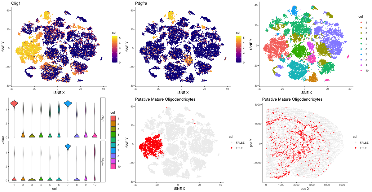
# markers of interest
markers <- c('Olig1', 'Olig2', 'Pdgfra', 'Osp', 'Mbp', 'Mog', 'Sox10')
markers.have <- intersect(markers, colnames(mat))
markers.have
gs.plot <- lapply(markers.have, function(g) {
df1 <- data.frame(x = emb[,1],
y = emb[,2],
col = mat[,g])
p1 <- ggplot(data = df1,
mapping = aes(x = x, y = y)) +
geom_scattermore(mapping = aes(col = col),
pointsize=1) +
scale_color_viridis_c(option = "plasma")
plot1 <- p1 + labs(x = "tSNE X" , y = "tSNE Y", title=g) +
theme_classic()
return(plot1)
})
gs.plot[1]
gs.plot[2]
set.seed(0)
clus <- kmeans(pcs$x[,1:30], centers = 10)$cluster
df1 <- data.frame(x = emb[,1],
y = emb[,2],
col = as.factor(clus))
p1 <- ggplot(data = df1,
mapping = aes(x = x, y = y)) +
geom_scattermore(mapping = aes(col = col),
pointsize=1)
plot1 <- p1 + labs(x = "tSNE X" , y = "tSNE Y") +
theme_classic()
plot1
df <- reshape2::melt(
data.frame(id=rownames(mat),
mat[, markers.have],
col=as.factor(clus)))
diffgexp.plot <- ggplot(data = df,
mapping = aes(x=col, y=value, fill=col)) +
geom_violin() +
theme_classic() +
facet_grid(variable ~ .)
diffgexp.plot
df2 <- data.frame(x = emb[,1],
y = emb[,2],
col = as.factor(clus==1))
p2 <- ggplot(data = df2,
mapping = aes(x = x, y = y)) +
geom_scattermore(mapping = aes(col = col),
pointsize=1)
plot2 <- p2 + labs(x = "tSNE X" , y = "tSNE Y",
title='Putative Mature Oligodendricytes') +
scale_color_manual(values=c("#eeeeee", "#FF0000")) +
theme_classic()
plot2
df3 <- data.frame(x = pos[,1],
y = pos[,2],
col = as.factor(clus==1))
p3 <- ggplot(data = df3,
mapping = aes(x = x, y = y)) +
geom_scattermore(mapping = aes(col = col),
pointsize=1)
plot3 <- p3 + labs(x = "pos X" , y = "pos Y",
title='Putative Mature Oligodendricytes') +
scale_color_manual(values=c("#eeeeee", "#FF0000")) +
theme_classic()
plot3
png("jfan9_MERFISH_matolig.png", width = 1200, height = 620)
gridExtra::grid.arrange(gs.plot[[1]], gs.plot[[2]],
plot1, diffgexp.plot,
plot2, plot3, ncol=3)
dev.off()
|