Mature Oligodendrocytes in MERFISH Data Predicted by high Olig1 expression and low or no Pdgfra expression

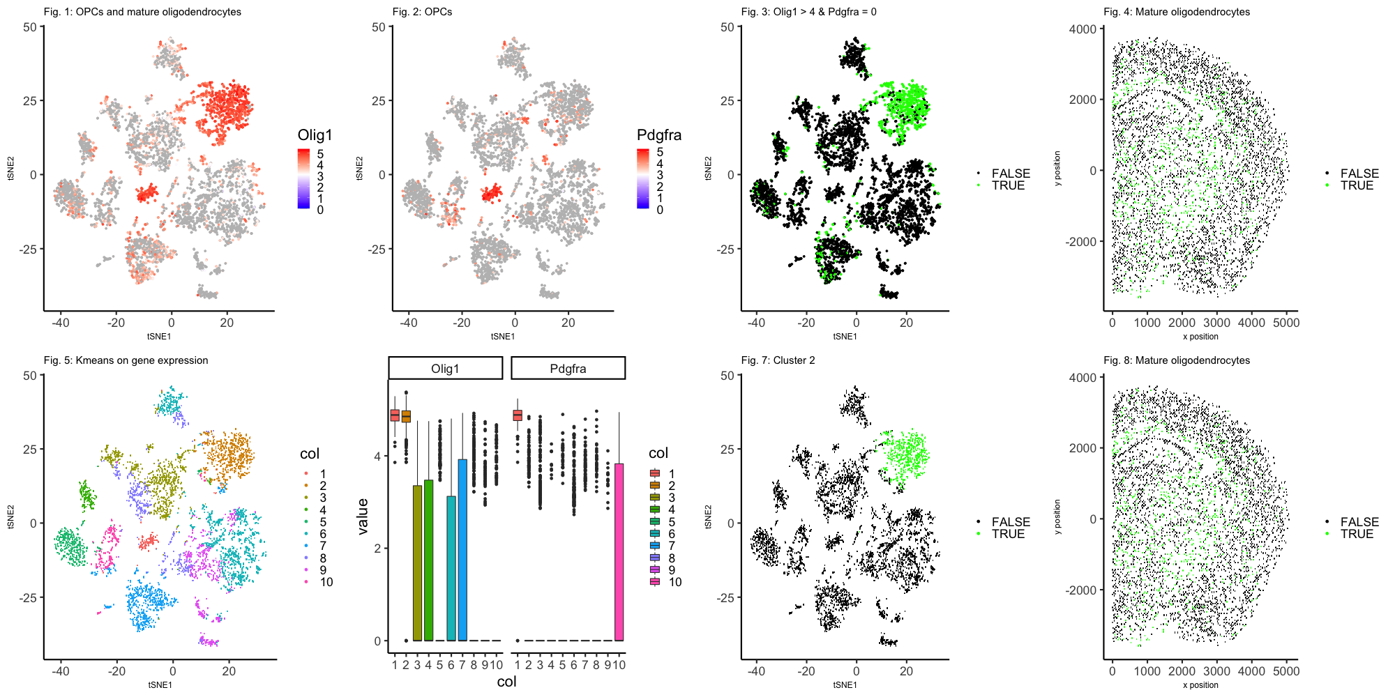
Gene expression of 5000 cells was measured by MERFISH. Initially, populations were grouped by the first thirty principle components and visualized in two dimensions by tSNE. Two populations of cells are shown to have high expression of oligodendrocyte marker Olig1 (Figure 1). Olig1 is known to be highly expressed in both oligodendrocyter progenitor cells (OPCs) and mature oligodendrocytes. Only one population is marked by high expression of Pdgfra (Figure 2). Pdgfra can be used to distinguish OPCs from mature oligodendrocytes since it is highly expressed in OPCs, but not expressed in mature oligodendrocytes. The population that both highly expresses Olig1 (> 10^4 counts per million) and does not express Pdgfra is predicted to be mature oligodendrocytes (Figure 3). These predicted mature oligodendrocytes, a type of glial, are distributed throughout the white matter (Figure 4). In a secondary analysis, the sample cells were grouped by kmeans clustering into ten clusters and visualized in two dimensions by tSNE (Figure 5). For all clusters, expression levels of Olig1 and Pdgfra were summarized as boxplots. The median expression of Olig1 is high in both cluster 1 and cluster 2. However, cluster 1 has high median expression of Pdgfra as well (Figure 6). By this analysis, cluster 2 is predicted to be mature oligodendrocytes (figure 7). These predicted mature oligodendrocytes also seem to be located in the white matter (Figure 8).
References:
- https://www.ncbi.nlm.nih.gov/pmc/articles/PMC6912544/
- https://stackoverflow.com/questions/28243514/ggplot2-change-title-size
#load libraries
library(Rtsne)
library(ggplot2)
library(scattermore)
library(gridExtra)
library(reshape2)

#load MERFISH data
data <- read.csv('~/Dropbox/JHU/Courses/genomic-data-visualization/data/MERFISH_Slice2Replicate2_halfcortex.csv.gz')

#downsample to 5000
set.seed(0)
vi <- sample(data[,1],5000)
ds <- data[data$X %in% vi,]

#make matrix of position
pos <- ds[, c('x','y')]
rownames(pos) <- ds[,1]

#make matrix of gene expression data without position
gexp <- ds[, 4:ncol(ds)]
rownames(gexp) <- ds[,1]

#CPM normalize
numgenes <- rowSums(gexp)
normgexp <- gexp/numgenes*1e6

#add pseudocounts to do log
mat <- log10(normgexp+1)

#############
#check that genes of interest are in matrix

#canonical mature oligodendrocytes genes
#but also expressed by oligodendrocyte Progenitor Cells (OPCs)
'Olig1' %in% colnames(mat)
'Olig2' %in% colnames(mat)
'Olig3' %in% colnames(mat)

#other genes mature oligodendrocytes express but not exclusive to them
'Osp' %in% colnames(mat)
'Mbp' %in% colnames(mat)
'Mog' %in% colnames(mat)
'Sox10' %in% colnames(mat)

#gene expressed by OPCs but not mature oligodendrocytes
'Pdgfra' %in% colnames(mat)

#only two genes of interest in matrix Olig1 and Pdgfra

# histogram of Olig1 expression among cells
histdf <- data.frame(mat)
phist1 <- ggplot(data = histdf,
                mapping = aes(x = Olig1)) +
  geom_histogram(mapping = aes(fill = histdf['Olig1'] > 0), bins = 20) +
  scale_fill_manual("Olig1>0",values = c("gray", "red")) +
  labs(title="Histogram Olig1", x="log10(Olig1+1)", y = "count")

# histogram of Pdgfra expression among cells
phist2 <- ggplot(data = histdf,
                 mapping = aes(x = Pdgfra)) +
  geom_histogram(mapping = aes(fill = histdf['Pdgfra'] > 0), bins = 20) +
  scale_fill_manual("Pdgfra>0",values = c("gray", "red"))	+
  labs(title="Histogram Pdgfra", x="log10(Pdgfra+1)", y = "count")

#grid.arrange(phist1, phist2, ncol=2)

###############
#PCA
pcs <-prcomp(mat)
df <- data.frame(x=c(1:30), y=pcs$sdev[1:30])
p <- ggplot(data = df,mapping = aes(x=x,y=y) ) + geom_line() +
  labs(title="Principle Components", x="index", y = "standard deviation")
#p

###############
# tSNE
set.seed(0)
emb <- Rtsne(pcs$x[,1:30], dims=2, perplexity = 30)$Y
rownames(emb) <- rownames(mat)
#head(emb)
#dim(emb)

#plot tSNE of PCs 1:30 colored by Olig1 expression
#set up color gradient
#cells with no expression are excluded as gray
#high expression is noticeable within the dynamic range of red saturation
#i.e. gray is zero, blue is 0 to 3, white is 3, and red is 3 to max
v <- c(0, 0.01, 3/max(mat[,'Olig1']), 1)
high_exp_col <- c("gray", "blue", "white","red")

df1 <- data.frame(x=emb[,1],
                  y=emb[,2],
                  col = mat[,'Olig1'])

p1 <- ggplot(data=df1, mapping = aes(x=x, y=y)) +
  geom_point(mapping = aes(col = col), size=1) +
  theme_classic(base_size=22) +
  scale_color_gradientn("Olig1", colours = high_exp_col, values = v) +
  labs(title="Fig. 1: OPCs and mature oligodendrocytes", x = "tSNE1" , y = "tSNE2") +
  theme(axis.title=element_text(size=12), plot.title = element_text(size=15))

#p1

#plot tSNE of PCs 1:30 colored by Pdgfra expression
#set up color gradient
#cells with no expression are excluded as gray
#high expression is noticeable within the dynamic range of red saturation
#i.e. gray is zero, blue is 0 to 3, white is 3, and red is 3 to max
v <- c(0, 0.01, 3/max(mat[,'Pdgfra']), 1)
high_exp_col <- c("gray", "blue", "white","red")

df2 <- data.frame(x=emb[,1],
                  y=emb[,2],
                  col = mat[,'Pdgfra'])

p2 <- ggplot(data=df2, mapping = aes(x=x, y=y)) +
  geom_point(mapping = aes(col = col), size=1) +
  theme_classic(base_size=22) +
  scale_color_gradientn("Pdgfra", colours = high_exp_col, values = v) +
  labs(title="Fig. 2: OPCs", x = "tSNE1" , y = "tSNE2")+
  theme(axis.title=element_text(size=12), plot.title = element_text(size=15))
#p2

#grid.arrange(phist1, p1, phist2, p2, ncol=2)


#plot tSNE of PCs 1:30 colored by predicted mature oligodendrocytes classification
df3 <- data.frame(x=emb[,1],
                  y=emb[,2],
                  col = mat[,'Olig1'] > 4 & mat[,'Pdgfra'] ==0)

p3 <- ggplot(data=df3, mapping = aes(x=x, y=y)) +
  geom_point(mapping = aes(col = col), size=1) +
  theme_classic(base_size=22) +
  scale_color_manual("", values = c("black","green")) +
  labs(title="Fig. 3: Olig1 > 4 & Pdgfra = 0", x = "tSNE1" , y = "tSNE2")+
  theme(axis.title=element_text(size=12), plot.title = element_text(size=15))
#p3


#plot position of cells colored by predicted mature oligodendrocytes classification
df4 <- data.frame(x = pos[,1],
                  y = pos[,2],
                  mature_olig = mat[,'Olig1'] > 4 & mat[,'Pdgfra'] ==0)
p4 <- ggplot(data = df4, mapping = aes(x = x, y = y)) +
  geom_scattermore(mapping = aes(col = mature_olig), pointsize=1) +
  scale_color_manual("", values = c("black","green")) +
  theme_classic(base_size=22) +
  labs(title="Fig. 4: Mature oligodendrocytes", x = "x position" , y = "y position")+
  theme(axis.title=element_text(size=12), plot.title = element_text(size=15))

#grid.arrange(p1, p2, p3, p4, ncol=4)

###############
# kmeans on gene expression
set.seed(0)
com <- kmeans(mat, centers=10)

#plot kmeans clusters
dfk <- data.frame(x = emb[,1],
                 y = emb[,2],
                 col = as.factor(com$cluster))
pk <- ggplot(data = dfk,
            mapping = aes(x = x, y = y)) +
  geom_scattermore(mapping = aes(col = col),
                   pointsize=1) + theme_classic(base_size=22) +
  labs(title="Fig. 5: Kmeans on gene expression", x = "tSNE1" , y = "tSNE2") +
  theme(axis.title=element_text(size=12), plot.title = element_text(size=15))
#pk

#grid.arrange(p1, p2, p3, pk, ncol=2)

# predicted cluster 2 is mature oligodendrocytes
# store vector of whether cells are in cluster 2
cluster_pred <- com$cluster == 2

## wilcox test on all genes for cells in cluster 2 against all other cells
## save the pvalues
pvs <- sapply(colnames(mat), function(g) {
  x = wilcox.test(mat[cluster_pred, g], mat[!cluster_pred, g],
                  alternative='two.sided')
  return(x$p.value)
})
## correct for multiple testing
table(p.adjust(pvs) < 0.05)
table(pvs < 0.05)

## calculate fold changes
fcs <- sapply(colnames(mat), function(g) {
  x = mean(mat[cluster_pred, g])/mean(mat[!cluster_pred, g])
  return(x)
})

# return p value and fold change for Olig1 for cells in cluster 10 against all other cells
# expect low p-value and fold change > 1
pvs["Olig1"]
fcs["Olig1"]

# return p value and fold change for Pdgfra for cells in cluster 10 against all other cells
# expect high p-value and fold change < 1
pvs["Pdgfra"]
fcs["Pdgfra"]

# Box plots for expression of Olig1 and Pdgfra in each cluster
dfcs <- reshape2::melt(
  data.frame(id=rownames(mat),
             mat[, c('Olig1','Pdgfra')],
             col=as.factor(com$cluster)))

pcs <- ggplot(data = dfcs,
       mapping = aes(x=col, y=value, fill=col)) +
  geom_boxplot() +
  theme_classic(base_size=22) +
  facet_wrap(~ variable)
#pcs

# plot predicted mature oligodendrocytes cluster
dfmo <- data.frame(x = emb[,1],
                  y = emb[,2],
                  col = cluster_pred)
pmo <- ggplot(data = dfmo,
             mapping = aes(x = x, y = y)) +
  geom_scattermore(mapping = aes(col = col),
                   pointsize=1) + theme_classic(base_size=22) +
  scale_color_manual("", values = c("black","green")) +
  labs(title="Fig. 7: Cluster 2", x = "tSNE1" , y = "tSNE2") +
  theme(axis.title=element_text(size=12), plot.title = element_text(size=15))
#pmo


#plot position of cells colored by predicted mature oligodendrocytes classification
dfpo <- data.frame(x = pos[,1],
                  y = pos[,2],
                  mature_olig = cluster_pred)
ppo <- ggplot(data = df4, mapping = aes(x = x, y = y)) +
  geom_scattermore(mapping = aes(col = mature_olig), pointsize=1) +
  scale_color_manual("", values = c("black","green")) +
  theme_classic(base_size=22) +
  labs(title="Fig. 8: Mature oligodendrocytes", x = "x position" , y = "y position") +
  theme(axis.title=element_text(size=12), plot.title = element_text(size=15))

png("HW4.png", width = 2000, height = 1000)
grid.arrange(p1, p2, p3, p4, pk, pcs, pmo, ppo, ncol=4)
dev.off()