Identifying the Cell-type of a Random Cell Cluster

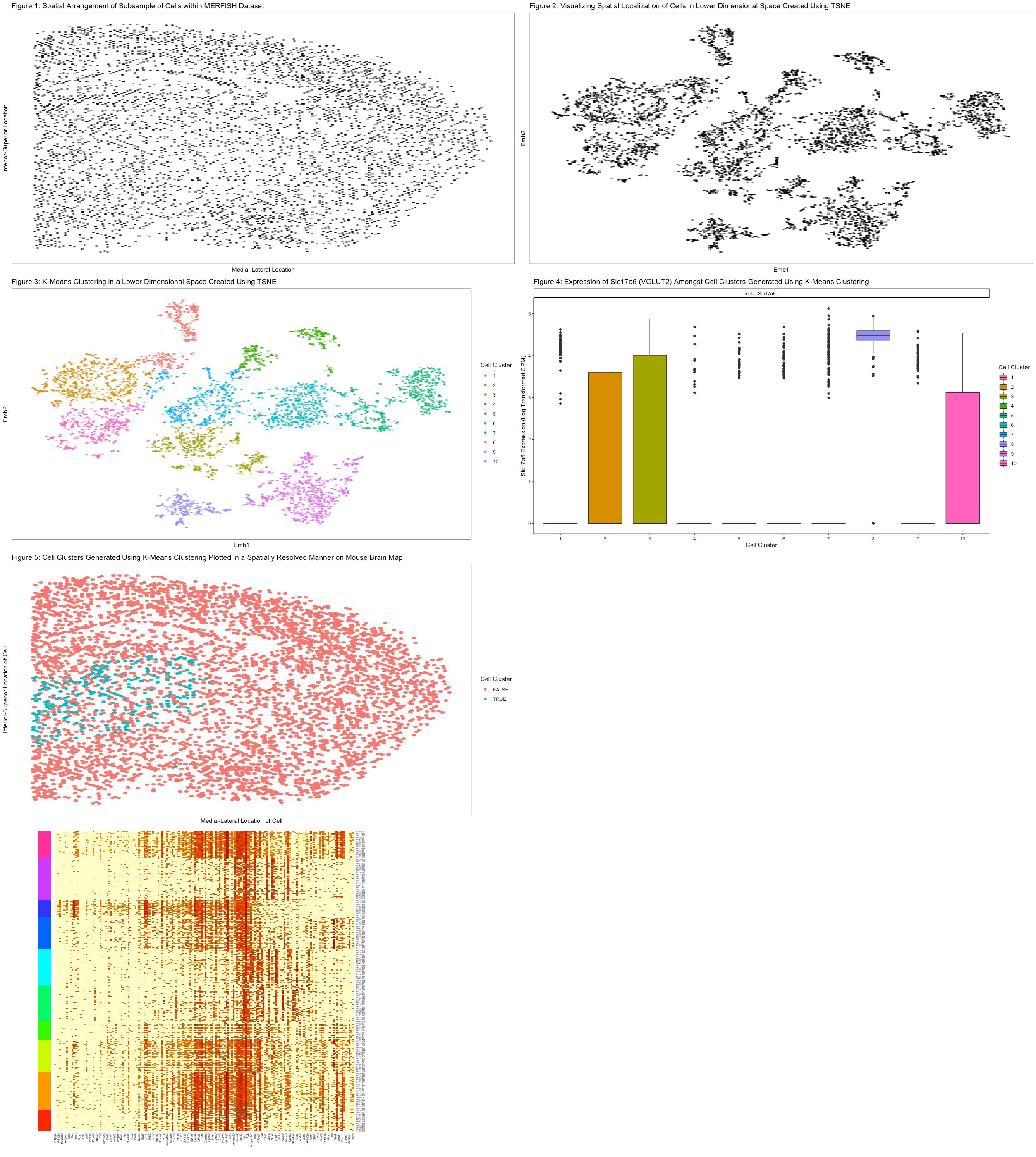
In Figure 1, I have plotted the spatial distribution of cells within our MERFISH data set, after down-sampling the data. I used the geometric primitive of points to represent single cells within our MERFISH dataset. I used the visual channel of position along the x and y axes to encode the respective positions of cells across the mouse brain. Clearly, from this data visualization, we make more salient the point that down-sampling faithfully mirrors the original tissue from which the data was derived.
In Figure 2, I performed TSNE analysis (non-linear dimensional reduction) on principal components 1 through 15, creating a 2-dimentional space derived from PC-space. I used the geometric primitive of points to represent single cells within our MERFISH dataset. I also utilized the visual channel of position along the x and y axes to cluster cells based on transcriptional similarity. Ultimately, the purpose of this data visualization is to show that cells form distinct groupings in the embedded space. This point is made poignantly given that cells, as indicated by points, can be grouped according to the Gestalt principle of grouping by proximity.
In Figure 3, I performed K-means clustering on the embedded space derived using TSNE. The geometric primitive of points was used to represent cells in the reduced dimensional space. Again, the visual channel of position along the x and y axes represents the grouping of cells based on transcriptional similarity. The channel of color, specifically hue, was used to encode the cell clusters generated using K-means clustering. The purpose of this figure is to demonstrate that there are specific cell-clusters in our data set, and this point is strengthened by the Gestalt principle of grouping by similarity in color.
After generating these cell clusters, I decided to further study cluster 8. I compared this cluster to the rest of the data set and found—using a “for loop”—that the expression of Slc17a6, Grm1/4, and Gbbr1/2 was upregulated significantly. Since Slc17a6 encodes VGLUT2 (vesicular glutamate transporter 2) and Grm1/4 and Gbbr1/2 encode glutamate and GABA receptors (respectively), I concluded that this cluster corresponds to a specific set of glutamatergic neurons, which receive both excitatory and inhibitory inputs. Then, in figure 4, I used box plots to demonstrate that VGLUT2 expression was indeed upregulated specifically within cluster 8. I used the geometric primitive of areas, and the visual channel of position along the y-axis corresponded to level of expression of Slc17a6, while the position along the x-axis corresponded to the cell cluster. Furthermore, the visual channel of hue was utilized to also represent cell cluster. Overall, the box plots make more salient that Slc17a6 is significantly upregulated in cluster 8 compared to the rest of the dataset.
In Figure 5, we projected the cell clusters derived from k-means clustering onto the original mouse brain map to identify the spatial location of our cluster of interest. Poignantly, I made all the cells outside of cluster 8 red in color while all the cells within cluster 8 were blue in color (using visual channel of hue here). Furthermore, the visual channel of position along the x and y axes represents the respective positions of cells across the mouse brain. As before, I used the geometric primitive of points to represent cells. All in all, it appears from this data visualization that this particular cluster of glutamatergic neurons, blue in color, is situated predominantly within the limbic system. This point is made more salient due to the use of Gestalt principle of grouping by similarity in color.
At the very end, I have attached a heat map showing the differentially expressed in cluster 8, which we have affirmed corresponds to a specific cluster of glutamatergic neurons in the brain, relative to the other clusters.
#Goal: Generate cell clusters from our MERFISH dataset and use differentially expressed genes to identify the cell type of said cell cluster.


data <- read.csv("/Users/ares2081/Desktop/MERFISH_Slice2Replicate2_halfcortex.csv")
pos <- data[, c('x', 'y')]
rownames(pos) <- data[,1]
gexp <- data[, 4:ncol(data)]
rownames(gexp) <- data[,1]


#Down-sample cells
j <- sample(rownames(pos), 5000)
pos <- pos[j,]
gexp <- gexp[j, ]
df0 <- data.frame(x = pos$x, y = pos$y)
library(scattermore)
p0 <- ggplot(data = df0,
             mapping = aes(x = x, y = y)) +
  geom_scattermore(mapping = NULL, pointsize=0.75) +
  ggtitle("Figure 1: Spatial Arrangement of Subsample of Cells within MERFISH Dataset") +
  labs(x = "Medial-Lateral Location", y = "Inferior-Superior Location") + theme_bw() + theme(panel.grid.major = element_blank(),
                                                    panel.grid.minor = element_blank(), axis.ticks.x=element_blank(),
                                                    axis.text.x=element_blank(), axis.ticks.y=element_blank(),axis.text.y=element_blank())
p0

#CPM normalize
numgenes <- rowSums(gexp)
normgexp <- gexp/rowSums(gexp)*1e6


#PCA (linear dimension reduction)
mat <- log10(normgexp+1)
pcs <- prcomp(mat)
names(pcs)
dim(pcs$x)
plot(pcs$sdev[1:30], type='l')
#It appears the first 15 PCs capture most of the standard deviation.
#Plotting the first 3 PCs, we see they don't truly capture all of the variation in our transcriptomic data.
library(ggplot2)
df1 <- data.frame(pc1 = pcs$x[,1],
                  pc2 = pcs$x[,2],
                  col = pcs$x[,3])
p1 <- ggplot(data = df1,
             mapping = aes(x = pc1, y = pc2)) +
  geom_point(mapping = aes(col=col))
p1

#Consequently, let's apply a non-linear dimensional reduction to our PCs (TSNE).
library(Rtsne)
set.seed(0)
emb <- Rtsne(pcs$x[, 1:15], dims=2, perplexity = 30)$Y
rownames(emb) <- rownames(mat)
#Plot MERFISH data in reduced 2-dimensional space
df2 <- data.frame(x = emb[,1], y = emb[,2])
p2 <- ggplot(data = df2,
             mapping = aes(x = x, y = y)) +
  geom_scattermore(mapping = NULL, pointsize=0.75) +
  ggtitle("Figure 2: Visualizing Spatial Localization of Cells in Lower Dimensional Space Created Using TSNE") +
  labs(x = "Emb1", y = "Emb2") + theme_bw() + theme(panel.grid.major = element_blank(),
                                                    panel.grid.minor = element_blank(), axis.ticks.x=element_blank(),
                                                    axis.text.x=element_blank(), axis.ticks.y=element_blank(),axis.text.y=element_blank())
p2


#K-means clustering in embedding space
set.seed(0)
com <- kmeans(emb, centers=10)
#Number of centers selected on the basis of number of groups seen in lower dimensional spatial visualization
df3 <- data.frame(x = emb[,1],
                  y = emb[,2],
                  col = as.factor(com$cluster))
p3 <- ggplot(data = df3,
             mapping = aes(x = x, y = y)) +
  geom_scattermore(mapping = aes(col = col), pointsize=0.75) +
  ggtitle("Figure 3: K-Means Clustering in a Lower Dimensional Space Created Using TSNE") +
  labs(x = "Emb1", y = "Emb2", color = "Cell Cluster") + theme_classic() + theme_bw() + theme(panel.grid.major = element_blank(),
                                                                                                    panel.grid.minor = element_blank(), axis.ticks.x=element_blank(),
                                                                                                    axis.text.x=element_blank(), axis.ticks.y=element_blank(),axis.text.y=element_blank())
p3


#Cluster 8 appears to be relatively isolated from other clusters, so let's run a "for loop" to identify differentially expressed cells in cluster 2.
#Let our starting gene for the for loop be Cx3cr1, which is a marker for microglia, and then iteratively, we can determine which genes are upregulated or downregulated in cluster 2.
g <- 'Cx3cr1'
viii <- com$cluster == 8
p_values <- sapply(colnames(mat), function(g) {
  x = wilcox.test(mat[viii, g], mat[!viii, g],
                  alternative='two.sided')
  return(x$p.value)
})
#Since we are running the Wilcoxon test iteratively, we will need to apply a Bonferroni correction to account for false significant results.
adusted <- p.adjust(p_values)
#Compute fold changes for all genes, comparing cluster 8 to the rest of the data set
fold_changes <- sapply(colnames(mat), function(g) {
  x = mean(mat[viii, g])/mean(mat[!viii, g])
  return(x)
})
#Generate heatmap of differentially expressed genes.
n <- names(which(adusted < 0.05))
n <- names(sort(fold_changes[n], decreasing=TRUE))
m <- mat[names(sort(com$cluster)),n]
col = rainbow(10)[as.factor(com$cluster)]
names(col) <- names(com$cluster)
heatmap(as.matrix(m), Rowv=NA, Colv=NA, scale='none',
        RowSideColors = col[rownames(m)])
#Clearly, cluster 8 is very distinct in terms of the genes it expresses compared to the rest of the clusters.

#Manually identify most upregulated genes in cell cluster 2 for the purpose of identification of cell-type.
a <- 'Cx3cr1'
p_values2 <- sapply(colnames(mat), function(a) {
  x = wilcox.test(mat[viii, a], mat[!viii, a],
                  alternative='greater')
  return(x$p.value)
})
sorted_diff <- sort(-log10(p.adjust(p_values2)), decreasing=TRUE)
sorted_diff[1:20]
#Most upregulated genes: Slc17a6, Vipr2, Adra2b, Adra1b, Grm4, Opn3, F2r, Grm1, Adgra1, Ret, Gabbr2, Hrh3, Gabbr1, Epha8, Gpr153, Flt3, Epha4, Gpr63, Fzd10, Lgr5
#It appears cluster 8 has high expression of Slc17a6, Grm1/4, and Gabbr1/2, based on the heatmap (where the blue band corresponds to cluster 8) and the upregulated gene analysis above.
#Importantly, Slc17a6 encodes VGLUT2, vesicular glutamate transporter 2, which is specific to glutamatergic neurons.
#Grm1/4 encode metabotropic glutamate receptors, while Gabbr1/2 encode GABA receptors. This affirms that this cluster consists of neurons, specifically glutamatergic neurons.


#Show that Slc17a6 is enriched in cluster 8 specifically
df4 <- reshape2::melt(
  data.frame(id=rownames(mat),
             mat[, 'Slc17a6'],
             col=as.factor(com$cluster)))
p4 <- ggplot(data = df4, mapping = aes(x=col, y=value, fill=col)) +
  geom_boxplot() + theme_classic() + facet_wrap(~variable) +
  ggtitle("Figure 4: Expression of Slc17a6 (VGLUT2) Amongst Cell Clusters Generated Using K-Means Clustering") +
  labs(x = "Cell Cluster", y = "Slc17a6 Expression (Log Transformed CPM)", fill = "Cell Cluster")
p4


#Plot clusters back onto original image of the brain
df5 <- data.frame(x = pos[,1],
                  y = pos[,2],
                  col = viii)
p5 <- ggplot(data = df5, mapping = aes(x = x, y = y)) + geom_scattermore(mapping = aes(col = col), pointsize=2) +
  ggtitle("Figure 5: Cell Clusters Generated Using K-Means Clustering Plotted in a Spatially Resolved Manner on Mouse Brain Map") +
  labs(x = "Medial-Lateral Location of Cell", y = "Inferior-Superior Location of Cell", color = "Cell Cluster") + theme_classic() + theme_bw() + theme(panel.grid.major = element_blank(),
                                                                                                                           panel.grid.minor = element_blank(), axis.ticks.x=element_blank(),
                                                                                                                           axis.text.x=element_blank(), axis.ticks.y=element_blank(),axis.text.y=element_blank())
p5
#Cluster8, glutamatergic neurons, appear to be concentrated near the center (within the limbic system perhaps).


#Multi-panel generation (will add heatmap to the end of this multi-panel)
library(gridExtra)
grid.arrange(p0, p2, p3, p4, p5, ncol=2)