Analyze the CODEX dataset

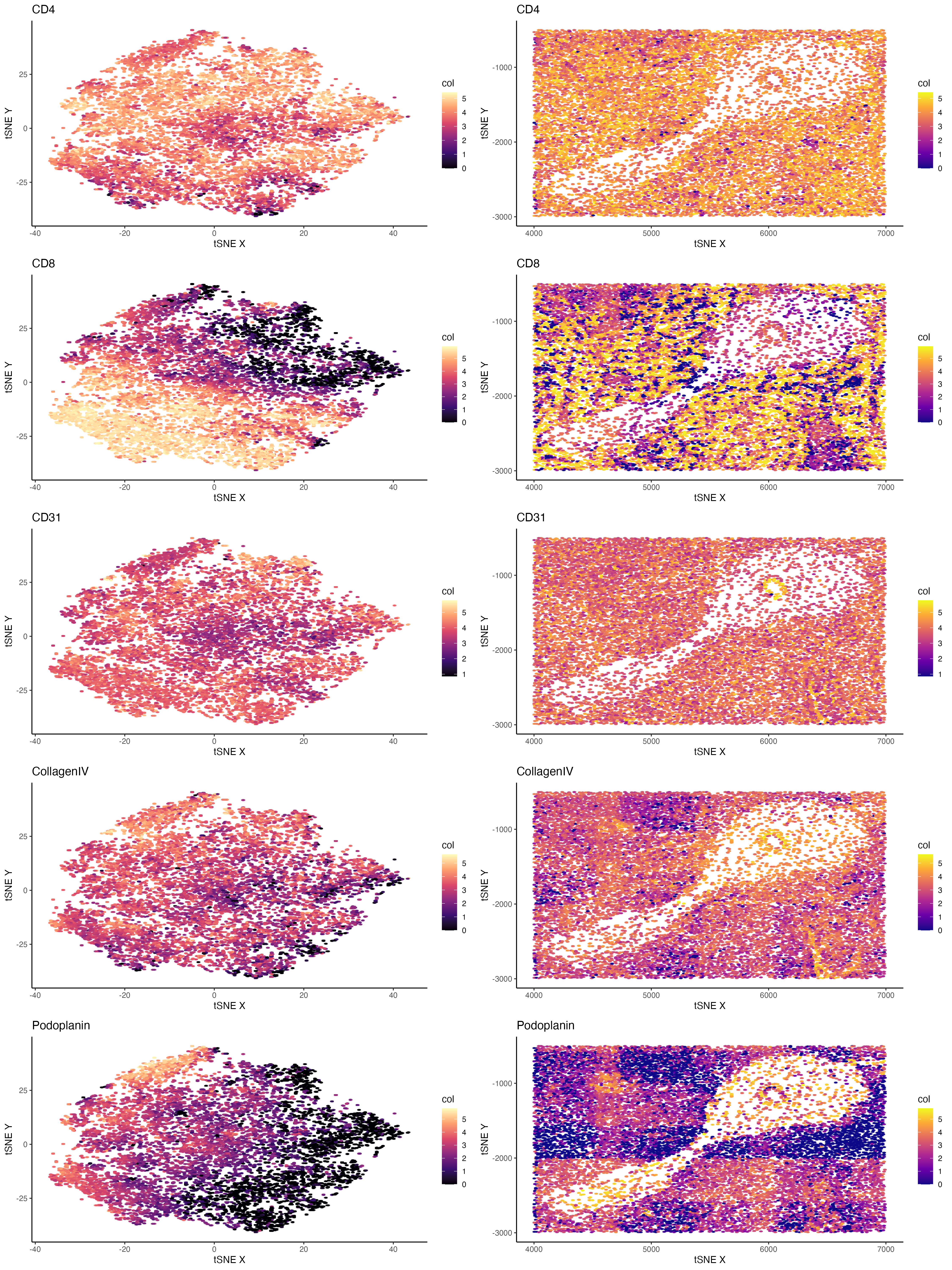
I tried to plot the protein expression in clusters and spatial organizations side by side for better comparison. I noticed a large proportion of genes sequenced are immune cell marker genes. For example, CD4( orCD8) and CD11b, which is canonical markers for T cell and B cell respectively. Thus, I have a quick quess that this is a biopsy of immune tissues. Furthermore, I want to look at the distributions of these proteins and ask questions like if they have specific organization patterns.

1) I noticed in the plotting that there are vascular endothelial cells (marked by CD31) forming small lumens indicating there are vessel structures. 2) Great majority of cells are expressing CD4. 3) CD8+ T cells (high CD8 expressing) are forming cord like structures. 4) Potential fibroblasts(high Collagen IV expressing) are dispersed in spaces of immune cells. 5) Podoplanin is a glycoprotein present primarily on the endothelium of lymphatic vessels. Thus I was more confirmed that the blank spaces with no cells present could possibly be crosssection of vessels.

By the visualizing how these cell-types are organized in the tissue, I could define that this tissue comes from an immune organs with rich vasculature and shows abundance in T cell, B cell and monocyte/marophage lineages. This tissue may be spleen.

library(Rtsne)
library(ggplot2)
library(scattermore)
library(gplots)
library(tidyverse)
library(kableExtra)
library(broom)
library(highcharter)
library(magrittr)
library(gridExtra)
library(cowplot)

data<- read.csv("codex_spleen_subset.csv.gz")
pos<-data[,2:3]
#get an overview of what the biopsy looks like
plot(pos,pch=".",cex=1)
area <- data[,4]
pexp <- data[, 5:ncol(data)]
colnames(pexp)
#normalization
numproteins <- rowSums(pexp)
normpexp <- pexp/numproteins*1e6
mat <- log10(normpexp+1)
#do PCA and tSNE based on pcs
pcs <- prcomp(mat)
plot(pcs$sdev[1:30], type="l")
set.seed(0)
emb <- Rtsne(pcs$x[,1:20], dims=2, perplexity=30)$Y

markers<-c("CD4","CD8","CD31","CollagenIV","Podoplanin")
pexp.plot <- lapply(markers, function(g) {
  df1 <- data.frame(x = emb[,1],
                    y = emb[,2],
                    col = mat[,g]) 
p1 <- ggplot(data = df1,
               mapping = aes(x = x, y = y)) +
    geom_scattermore(mapping = aes(col = col), 
                     pointsize=2) + 
    scale_color_viridis_c(option = "magma" ) 
  plot1 <- p1 + labs(x = "tSNE X" , y = "tSNE Y", title= g ) +
    theme_classic()
  return(plot1)
})


set.seed(0)
com <- kmeans(pcs$x[,1:20], centers = 10)
df1 <- data.frame(x = emb[,1],
                  y = emb[,2],
                  col = as.factor(clus$cluster)) 
ggplot(data = df1,
             mapping = aes(x = x, y = y)) +
  geom_scattermore(mapping = aes(col = col), 
                   pointsize=2)

# To determine what tissue it is, I want to look at spatial distributions of these proteins.

pos.plot <- lapply(markers, function(g) {
  df2 <- data.frame(x = pos[,1],
                 y = pos[,2],
                 col = mat[,g]) 
p1 <- ggplot(data = df2,
               mapping = aes(x = x, y = y)) +
    geom_scattermore(mapping = aes(col = col), 
                     pointsize=2) + 
    scale_color_viridis_c(option = "plasma") 
  plot1 <- p1 + labs(x = "tSNE X" , y = "tSNE Y", title= g ) +
    theme_classic()
  return(plot1)
})



row_1<- plot_grid( pexp.plot[[1]],pos.plot[[1]],ncol=2, nrow=1)
row_2<- plot_grid( pexp.plot[[2]],pos.plot[[2]],ncol=2, nrow=1)
row_3<- plot_grid( pexp.plot[[3]],pos.plot[[3]],ncol=2, nrow=1)
row_4<- plot_grid( pexp.plot[[4]],pos.plot[[4]],ncol=2, nrow=1)
row_5<- plot_grid( pexp.plot[[5]],pos.plot[[5]],ncol=2, nrow=1)

plot_grid(row_1,row_2,row_3,row_4,row_5,nrow=5)

ggsave("Stella_Li.png",width=15,height =20 )