Captions:

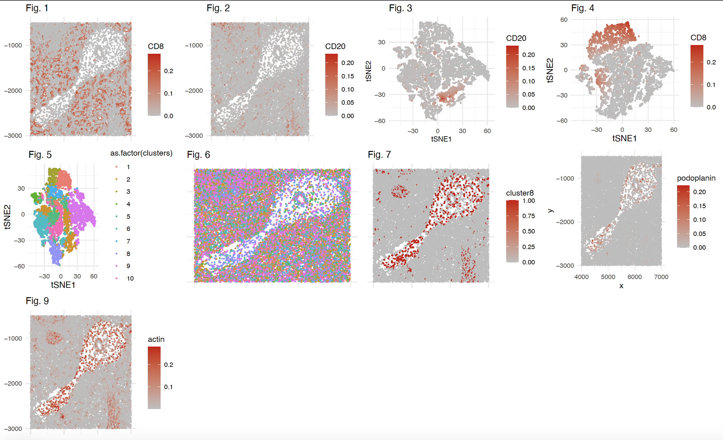
Fig 1: Spatial localization of normalized CD8 abundance in CODEX dataset. The 8 Proteins with the least varying abudance (Var< 1.141120e-04 on the normalized dataset, this is arbitrary and I felt that other proteins might be sufficient to identify the tissue) were removed from the dataset for further analysis. Normalization was performed by dividing fluorescence intensity values by cell 2D area and total protein intensity found in the cell. CD8 is a protein found in T cells. Appears to be little CD8+ cells outside of the relatively acellular region of the section.

Fig 2: Spatial localization of normalized (described above) CD20 abundance in CODEX dataset. CD20 is a protein found in B cells. Appears to be minimal CD20+ cells inside of the relatively acellular region of the section.

Fig 3: tSNE was performed on the filtered and normalized dataset to visualize the data in low dimensions. Cells were colored by normalized abundance of CD20 to visualize clusters or cells that express CD20. Appears to be minimal CD20+ cells inside of the relatively acellular region of the section.

Fig 4: tSNE was performed on the filtered and normalized dataset to visualize the data in low dimensions. Cells were colored by normalized abundance of CD8 to visualize clusters or cells that express CD8.

Fig 5: k-Means clustering (10 centroids) was performed on the filtered and normalized dataset. Cells were colored by their respective cluster identity in tSNE space.

Fig 6: Spatial distribution of 10 clusters as previously determined by k means clustering.

Fig 7: Visual of spatial distribution of cells, colored by cluster 8 identity to depict enrichment of cluster 8 cells in this relatively acellular region in the spleen.

Fig 8. (right of Fig. 7 in panel): Visual of spatial distribution of cells, colored by normalized Podoplanin protein abundance to depict some enrichment of Podoplanin in the cells in the relatively acellular region of this spleen section. In the spleen, podoplanin seems to be found in endothelial cells, which are localized in the Red Pulp of the spleen. Podoplanin abundance was significantly higher in cluster 8 cells compared to all other cells, as determined by a t-test.

Fig 9. Visual of spatial distribution of cells, colored by normalized Podoplanin protein abundance to depict some enrichment of Actin in the cells in the relatively acellular region of this spleen section. In the spleen, Actin seems to be found in smooth muscle cells, which are localized in the Red Pulp of the spleen. Actin abundance was significantly higher in cluster 8 cells compared to all other cells, as determined by a t-test.

Overall: I think this may be a red pulp/white pulp boundary of the spleen. The (somewhat) acellular region in the middle of the section seems to be enriched with cells expressing actin and podoplanin, which are found in the red pulp.

Localization of podoplanin in red pulp found using this paper:

https://www.researchgate.net/publication/5398375_Ly49H_NK_Cells_Migrate_to_and_Protect_Splenic_White_Pulp_Stroma_from_Murine_Cytomegalovirus_Infection/figures?lo=1

Further information that PDPN is localized in reticular and endothelial cells, which indicates localization in red pulp if we are looking at spleen https://www.researchgate.net/publication/224919228_A_Novel_Bacterial_Artificial_Chromosome-Transgenic_Podoplanin-Cre_Mouse_Targets_Lymphoid_Organ_Stromal_Cells_in_vivo

*I had discussed normalization with Kalen

```{r setup, include=FALSE} #to figure this out, I am first going to look online to find the cell types we are likely to find within spleen and proteins that are commonly used to detect them.

#found this article: #Normal Structure, Function, and Histology of the Spleen #https://journals.sagepub.com/doi/full/10.1080/01926230600867743

#two different types of architecture of the spleen that differ in their cell compositions, architecture and morphology:

- white pulp: lymphocytes, macrophages, dendritic cells, plasma cells, arterioles, and capillaries

- red pulp: platelets, granulocytes, red blood cells

#seems like white pulp should have more T cells and immune cells while red pulp should have more blood and leukocytes cells. lets plot and find out

library(tidyverse) set.seed(1)

#read in codex dataset codex=read.csv(‘codex_spleen_subset.csv’) rownames(codex)=codex$X codex$X=NULL

#start over. will still normalize by area codex_intensityonly=codex codex_intensityonly$x=NULL codex_intensityonly$y=NULL codex_intensityonly$area=NULL

#normalize intensity values for differences in cell area codex_intensityonly=codex_intensityonly/codex$area codex_intensityonly=codex_intensityonly/rowSums(codex_intensityonly)

codex_intensityonly=log10(codex_intensityonly+1) hist(apply(codex_intensityonly, 2, var))

#seems like there are some genes that have low variance. #removing 8 features with lowest variance low_var=sort(apply(codex_intensityonly, 2, var))[1:8] #lowest 8 are in the below list remove=c(‘PanCK’,’CD1c’,’CD35’,’CD11c’,’HLA.DR’,’CD21’,’CD5’,’CD45’)

for (i in remove){ codex_intensityonly[i]=NULL }

codex_intensityonly=log10(codex_intensityonly+1)

embedding=Rtsne(codex_intensityonly, dims=2, perplexity=20)$Y colnames(embedding)=c(‘tsne1’,’tsne2’)

embedding=data.frame(x = embedding[,1], y = embedding[,2]) embedding$CD20=codex_intensityonly$CD20 embedding$CD8=codex_intensityonly$CD8 embedding$CD31=codex_intensityonly$CD31 embedding$SMActin=codex_intensityonly$SMActin embedding$CD4=codex_intensityonly$CD4

#k means as well #only 8 visual channel clusters=kmeans(codex_intensityonly,centers = 10)

embedding[‘clusters’]=as.factor(clusters$cluster)

bcells=ggplot(data=embedding,mapping = aes(x = x, y = y)) +geom_point(mapping = aes(col =CD20),size=0.4)+xlab(‘tsne1’)+ylab(‘tsne2’)+theme_minimal()+scale_color_gradient2(low=”darkgrey”, mid=”grey”,high=”red3”)

tcells_cd8=ggplot(data=embedding,mapping = aes(x = x, y = y)) +geom_point(mapping = aes(col =CD8),size=0.4)+xlab(‘tsne1’)+ylab(‘tsne2’)+theme_minimal()+scale_color_gradient2(low=”darkgrey”, mid=”grey”,high=”red3”)

tcells_cd4=ggplot(data=embedding,mapping = aes(x = x, y = y)) +geom_point(mapping = aes(col =CD4),size=0.4)+xlab(‘tsne1’)+ylab(‘tsne2’)+theme_minimal()+scale_color_gradient2(low=”darkgrey”, mid=”grey”,high=”red3”)

kmeansclusters_tsne=ggplot(data=embedding,mapping = aes(x = x, y = y)) +geom_point(mapping = aes(col =as.factor(clusters)),size=0.5)+xlab(‘tsne1’)+ylab(‘tsne2’)+theme_minimal()

embedding$x=codex$x embedding$y=codex$y

cluster8=c() cluster1=c() cluster2=c() cluster3=c() cluster4=c() cluster5=c() cluster6=c() cluster7=c() cluster9=c() cluster10=c()

for (i in embedding$clusters){ if (i==8){ cluster8=c(cluster8,1)} else { cluster8=c(cluster8,0)} }

for (i in embedding$clusters){ if (i==9){ cluster9=c(cluster9,1)} else { cluster9=c(cluster9,0)} }

for (i in embedding$clusters){ if (i==1){ cluster1=c(cluster1,1)} else { cluster1=c(cluster1,0)} }

for (i in embedding$clusters){ if (i==2){ cluster2=c(cluster2,1)} else { cluster2=c(cluster2,0)} }

for (i in embedding$clusters){ if (i==3){ cluster3=c(cluster3,1)} else { cluster3=c(cluster3,0)} }

for (i in embedding$clusters){ if (i==4){ cluster4=c(cluster4,1)} else { cluster4=c(cluster4,0)} }

for (i in embedding$clusters){ if (i==5){ cluster5=c(cluster5,1)} else { cluster5=c(cluster5,0)} }

embedding[‘cluster8’]=cluster8 embedding[‘cluster9’]=cluster9 embedding[‘cluster1’]=cluster1 embedding[‘cluster2’]=cluster2 embedding[‘cluster3’]=cluster3 embedding[‘cluster4’]=cluster4 embedding[‘cluster5’]=cluster5

clusters_spatial=ggplot(embedding,aes(x,y))+geom_point(size=0.5,aes(col=clusters))+theme_minimal()+theme(legend.position=”none”)+ theme(axis.text.x=element_blank())+ theme(axis.text.y =element_blank(),axis.title.x=element_blank(), axis.title.y=element_blank())

#what is cluster 4? seems to be somewhat localized inside the enclosed region

clusters_spatial_8only=ggplot(embedding,aes(x,y))+geom_point(size=0.5,aes(col=cluster8))+theme_minimal()+ theme(axis.text.x=element_blank())+ theme(axis.text.y=element_blank(),axis.title.x=element_blank(),axis.title.y=element_blank())+scale_color_gradient2(low=”darkgrey”, mid=”grey”,high=”red3”)

codex_intensityonly[‘clusters’]=embedding$clusters vi=embedding$clusters==8

codex_intensityonly$clusters=NULL

pvs=sapply(colnames(codex_intensityonly), function(g) { x = wilcox.test(codex_intensityonly[vi, g], codex_intensityonly[!vi, g], alternative=’greater’) return(x$p.value)})

#strange p values. maybe my normalization method is wrong. # sort(pvs)[1:2] #seems like top 2 lowest p-values are SMActin and Podoplanin

actin=ggplot(data=embedding,mapping = aes(x = x, y = y)) +geom_point(mapping = aes(col =SMActin),size=0.4)+xlab(‘tsne1’)+ylab(‘tsne2’)+theme_minimal()+scale_color_gradient2(low=”darkgrey”, mid=”grey”,high=”red3”)

embedding[‘podoplanin’]=codex_intensityonly$Podoplanin embedding[‘actin’]=codex_intensityonly$SMActin embedding[‘CD8’]=codex_intensityonly$CD8 embedding[‘CD20’]=codex_intensityonly$CD20

podoplanin=ggplot(data=embedding,mapping = aes(x = x, y = y)) +geom_point(mapping = aes(col =podoplanin),size=0.4)+theme_minimal()+scale_color_gradient2(low=”darkgrey”, mid=”grey”,high=”red3”)+theme(axis.text.x=element_blank())+ theme(axis.title.x=element_blank(), axis.title.y=element_blank())

actin=ggplot(data=embedding,mapping = aes(x = x, y = y)) +geom_point(mapping = aes(col =actin),size=0.4)+theme_minimal()+scale_color_gradient2(low=”darkgrey”, mid=”grey”,high=”red3”)+theme(axis.text.x=element_blank())+ theme(axis.title.x=element_blank(), axis.title.y=element_blank())

cd8=ggplot(data=embedding,mapping = aes(x = x, y = y)) +geom_point(mapping = aes(col =CD8),size=0.4)+theme_minimal()+scale_color_gradient2(low=”darkgrey”, mid=”grey”,high=”red3”)+theme(axis.text.x=element_blank())+ theme(axis.title.x=element_blank(), axis.title.y=element_blank())

cd20=ggplot(data=embedding,mapping = aes(x = x, y = y)) +geom_point(mapping = aes(col =CD20),size=0.4)+theme_minimal()+scale_color_gradient2(low=”darkgrey”, mid=”grey”,high=”red3”)+theme(axis.text.x=element_blank())+ theme(axis.title.x=element_blank(), axis.title.y=element_blank())

#Using this paper: #https://www.researchgate.net/publication/5398375_Ly49H_NK_Cells_Migrate_to_and_Protect_Splenic_White_Pulp_Stroma_from_Murine_Cytomegalovirus_Infection/figures?lo=1

#I found that pdpn in spleen is usually used to show endothelial and reticular cells, which we are likely to find in the red pulp of the spleen

cd8_final=cd8+labs(title=”Fig. 1”)+theme(axis.title=element_text(size=12), plot.title = element_text(size=13))

cd20_final=cd20+labs(title=”Fig. 2”)+theme(axis.title=element_text(size=12), plot.title = element_text(size=13))

bcells_final=bcells+labs(title=”Fig. 3”, x = “tSNE1” , y = “tSNE2”)+theme(axis.title=element_text(size=10), plot.title = element_text(size=13))

tcells_final=tcells+labs(title=”Fig. 4”, x = “tSNE1” , y = “tSNE2”)+theme(axis.title=element_text(size=12), plot.title = element_text(size=13))

kmeans_final=kmeansclusters_tsne+labs(title=”Fig. 5”, x = “tSNE1” , y = “tSNE2”)+theme(axis.title=element_text(size=12), plot.title = element_text(size=13))

clusters_spatial_final=clusters_spatial+labs(title=”Fig. 6”)+theme(axis.title=element_text(size=12), plot.title = element_text(size=13))

clusters_spatial_8only_final=clusters_spatial_8only+labs(title=”Fig. 7”)+theme(axis.title=element_text(size=12), plot.title = element_text(size=13))

podoplanin_final=podoplanin+labs(title=”Fig. 8”)+theme(axis.title=element_text(size=12), plot.title = element_text(size=13))

actin_final=actin+labs(title=”Fig. 9”)+theme(axis.title=element_text(size=12), plot.title = element_text(size=13))

library(gridExtra)

grid.arrange(cd8_final, cd20_final, bcells_final, tcells_final,kmeans_final,clusters_spatial_final,clusters_spatial_8only_final,podoplanin,actin_final,ncol=4)

1
2