The effect of Count Per Million normalization on Dimensionality Reduction

What data types are you visualizing?

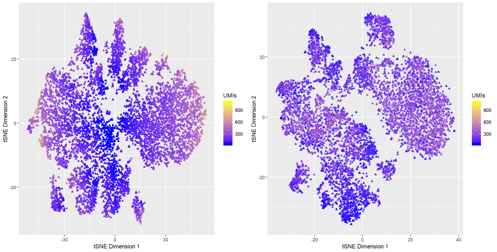
I am visualizing quantitative data of cells’ position on tSNE embedded 2-dimensional space. I am also visualizing the total gene count for each individual cell. Only cells with at least 1 UMI (unique molecular identifier) are displayed. I computed tSNE dimensionality reduction for both normalized gene counts and not-normalized gene counts and ploted them side by side.

What data encodings are you using to visualize these data types?

I am using the geometric primitive of points to represent cells. I used the visual channel of position along x- and y-axis to represent cells’ position in the t-SNE space. I used the visual channel of hue (diverging colors) and saturation (a continous gradient) to represent cells’ total gene count. Cells with low total gene count are colored blue, and cells with high gene counts are colored yellow.

What type of data visualization is this? What about the data are you trying to make salient through this data visualization?

My data visualization seeks to demonstrate that without normalization, tSNE dimensionality reduction tends to group cells with low gene count together. Cells with high gene counts are pushed outwards, as shown by gradients towards yellow color on the outer peripherals of the clusters. This means that gene-count is a factor that drives the similarity calculation at the high dimensional space.

However, varying total gene count can be attributed to imperfect technical practices, such as tissue slices not preserving the entirety of cells or errorneous segmentation. In addition, varying total gene count may also be attributed to biological variations such as cell cycles. Unless we are interested in exploring questions relating cell cycles, such confounding variable should be eliminated. While we could perform a cell-cycle imputation on the dataset at hand and then properly regress out the effect, if nothing else, we can at least normalize the dataset with methods such as counts per million (CPM).

We see that with normalization (figure on the right), yellow-colored points appear to evenly spread among clusters, thus server to mitigate our concerns to some extents.

What Gestalt principles or knowledge about perceptiveness of visual encodings are you using to accomplish this?

I am using gradients of colors to represent cells’ UMI counts. This visual encoding enables viewers to quickly see the trend I described above.

Code

library(ggplot2)
library(Rtsne)
library(gridExtra)

# Read in data
data <- read.csv("squirtle.csv.gz")
posn <- data[,2:3]
area <- data[,4]
gexp <- data[,5:ncol(data)]
rownames(posn) <- names(area) <- rownames(gexp) <- data[,1]

# Filter out all cells with no UMIs
UMIs <- rowSums(gexp)
valid<- UMIs > 0
posn <- posn[valid,]
area <- area[valid ]
gexp <- gexp[valid,]

# Normalization by Total Gene count within a cell
ratio_gexp <- gexp / rowSums(gexp)

# For reproducibility.
set.seed(0) 
emb1 <- Rtsne(gexp)

# For reproducibility.
set.seed(0) 
emb2 <- Rtsne(ratio_gexp)

# Plot cells on a tSNE embedded space, color cells by UMIs
df1 <- data.frame(emb1$Y, UMIs=UMIs[valid])
p1  <- ggplot(df1, aes(x=X1, y=X2, col=UMIs)) + 
  geom_point(shape=17) + 
  scale_color_gradient2(low="blue", high="yellow", mid="blue", midpoint=50) + 
  labs(x="tSNE Dimension 1", y="tSNE Dimension 2")

# Plot cells on a tSNE embedded space, color cells by UMIs
df2 <- data.frame(emb2$Y, UMIs=UMIs[valid])
p2  <- ggplot(df2, aes(x=X1, y=X2, col=UMIs)) + 
  geom_point(alpha=0.8, shape=17) + 
  scale_color_gradient2(low="blue", high="yellow", mid="blue", midpoint=50) + 
  labs(x="tSNE Dimension 1", y="tSNE Dimension 2")

# Place two plots side by side
grid.arrange(p1, p2, ncol=2)