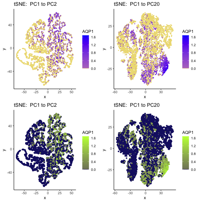
AQP1 Expression for Contrasting Principle Component Numbers
What data types are you visualizing?
I am using categorical data (zero and nonzero expression) as well as quantitative (color gradient of expression).
What data encodings are you using to visualize these data types?
My geometric primitive is a point for both my plots. My visual channels are position and color. Position encodes the values of the two tSNE dimensionality reduction features. Color (hue) encodes no AQP1 expression (gold for 1 / dark blue for 2) and AQP1 expression (blue/green). A midpoint color (purple / olive green) helps represent a lower (but still nonzero) expression (a higher expression being the primary color still).
What type of data visualization is this? What about the data are you trying to make salient through this data visualization?
My data visualization contains four tSNE plots that have two different numbers of principle components done on my charmander gene expression dataset. The gene I am focusing on is AQP1. The left two visualizations both display PC1->PC2 plots (just different colors and sizes to explore saliency contrast), while the right two visualizations display PC1 -> PC20 plots (with same color/size scheme). I wanted to explore how the saliency of my data clusters is impacted by the choice of how many PCA components are included. Note that I chose to normalize the gene data on a log10 scale prior to my PCA dimensionality reduction in an attempt to have more interpretable data clusters.
What Gestalt principles or knowledge about perceptiveness of visual encodings are you using to accomplish this?
My visualizations use the Gesalt principle of similarity (which is encoded by color/hue as described above) to aid the interpretation of groupings. Proximity was also chosen, and can be further expressed by more data normalization being conducted, which also aids in the interpreation of distinct groupings existing.
Code
library(ggplot2)
library(gridExtra)
library(Rtsne)
data <- read.csv('charmander.csv')
ds <- data
gexp <- data[, 4:ncol(data)]
rownames(gexp) <- ds[,1]
cellexp <- colSums(gexp != 0)
cdata <- data.frame(cellexp)
head(cellexp[order(cellexp, decreasing = TRUE)])
mat <- log10(gexp+1)
pcs <-prcomp(mat)
df <- data.frame(x=c(1:22), y=pcs$sdev[1:22])
# tSNE
set.seed(0)
emb <- Rtsne(pcs$x[,1:2], dims=2, perplexity = 20, check_duplicates = FALSE)$Y
rownames(emb) <- rownames(mat)
head(emb)
dim(emb)
df1 <- data.frame(x=emb[,1],
                  y=emb[,2],
                    col = mat[,'AQP1'])

p1 <- ggplot(data=df1, mapping = aes(x=x, y=y)) +
  geom_point(mapping = aes(col = col), size=0.5) +
  theme_classic() +
  scale_color_gradientn("AQP1", colours =
                          c(low = "lightgoldenrod", high = "blue"), values = c(0,0.01,1)) +
  labs(title="tSNE:  PC1 to PC2")

p1_2 <- ggplot(data=df1, mapping = aes(x=x, y=y)) +
  geom_point(mapping = aes(col = col), size=1.2) +
  theme_classic() +
  scale_color_gradientn("AQP1", colours =
                          c(low = "midnightblue", high = "olivedrab1"), values = c(0,0.01,1)) +
  labs(title="tSNE:  PC1 to PC2")

emb2 <- Rtsne(pcs$x[,1:20], dims=2, perplexity = 20, check_duplicates = FALSE)$Y
rownames(emb2) <- rownames(mat)
head(emb2)
dim(emb2)
df2 <- data.frame(x=emb2[,1],
                  y=emb2[,2],
                  col = mat[,'AQP1'])

p2 <- ggplot(data=df2, mapping = aes(x=x, y=y)) +
  geom_point(mapping = aes(col = col), size=0.5) +
  theme_classic() +
  scale_color_gradientn("AQP1", colours =
                          c(low = "lightgoldenrod", high = "blue"), values = c(0,0.01,1)) +
  labs(title="tSNE:  PC1 to PC20")

p2_2 <- ggplot(data=df2, mapping = aes(x=x, y=y)) +
  geom_point(mapping = aes(col = col), size=1.2) +
  theme_classic() +
  scale_color_gradientn("AQP1", colours =
                          c(low = "midnightblue", high = "olivedrab1"), values = c(0,0.01,1)) +
  labs(title="tSNE:  PC1 to PC20")

grid.arrange(p1, p2, p1_2, p2_2, ncol=2)

# color source: http://www.stat.columbia.edu/~tzheng/files/Rcolor.pdf
# I used the in-class PCA example as a starting template very early on
# This source https://distill.pub/2016/misread-tsne/ helped me choose a perplexity number

ggsave(filename = 'esimon10_hw3_gdv.png')