Homework 3 Submission: Comparing Pre-processing Methods Prior to PCA
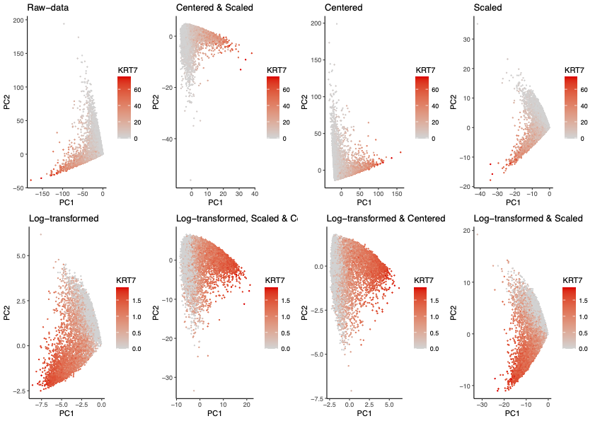
This series of plots demonstrates the effects of preprocessing steps taken prior to utilizing PCA for dimensionality reduction of multi-dimensional gene expression data. Some pre-processing steps include but is not limited to log-transforming the gene expression, centering the data at 0, scaling the data such that variance is 1, removing cells with 0 gene counts, and removing genes with 0 counts. In this series, I explored the effects of pre-processing methods such as scaling, centering, and log-transforming, and the combination of these methods.
The gene expression of KRT7 was utilized to highlight the expression profiles within each plot, and the corresponding scale for gene expression was chosen relative to whether the data had been log-transformed. Specifically, the distinct hues were chosen to indicate low and high expression of a gene that demonstrated high loading values in almost all PCAs, KRT7. Furthermore, the similarity of each cell is encoded in the spatial information of the x and y axis, exploiting Gestalt’s principle of proximity to group similar cells together. Lastly, I grouped plots that were not log-transformed together such that paired analysis between plots are easier to visualize.
1
2
3
4
5
6
7
8
9
10
11
12
13
14
15
16
17
18
19
20
21
22
23
24
25
26
27
28
29
30
31
32
33
34
35
36
37
38
39
40
41
42
43
44
45
46
47
48
49
50
51
52
53
54
55
56
57
58
59
60
61
62
63
64
65
66
67
68
69
70
71
72
73
74
75
76
77
78
79
80
81
82
83
84
85
86
87
88
89
90
91
92
93
94
95
data <- read.csv('/Users/ryanchan/Desktop/gdv_2023/data/bulbasaur.csv.gz', row.names = 1)
head(data)
data[1:5, 1:5]
?read.csv

gexp <- data[,4:ncol(data)]
gexp[1:5, 1:5]

totgenes <- rowSums(gexp)
good.cells <- names(totgenes)[totgenes > 0]
mat <- gexp[good.cells,]

gexp_raw <- mat
gexp_log <- log10(mat + 1)
gexp_cent <- scale(gexp_raw, center = TRUE, scale = FALSE)
gexp_scale <- scale(gexp_raw, center = FALSE, scale = TRUE)
gexp_cs <- scale(gexp_raw, center= TRUE, scale = TRUE)
gexp_norm_cs <- log10(gexp_raw + 1)
gexp_norm_cs <- scale(gexp_norm_cs, center = TRUE, scale = TRUE)
gexp_norm_c <- scale(gexp_log, center = TRUE, scale = FALSE)
gexp_norm_s <- scale(gexp_log, center = FALSE, scale = TRUE)

pcs_raw <- prcomp(gexp_raw, center = FALSE, scale. = FALSE)
plot(1:100, pcs_raw$sdev[1:100], type = "l")
head(sort(pcs_raw$rotation[,1], decreasing = TRUE))
head(sort(pcs_raw$rotation[,1], decreasing = FALSE))
df_raw <- data.frame(pcs_raw$x[,1:2], KRT7 = gexp_raw[,'KRT7'])
library(ggplot2)
p1 <- ggplot(data = df_raw, aes(x = PC1, y = PC2, col = KRT7)) +
  geom_point(size = 0.25) + scale_color_gradient(low = 'lightgrey', high = 'red') +
  theme_classic() + labs(title = "Raw-data")

pcs_log <- prcomp(gexp_log, center = FALSE, scale. = FALSE)
plot(1:100, pcs_log$sdev[1:100], type = "l")
head(sort(pcs_log$rotation[,1], decreasing = TRUE))
head(sort(pcs_log$rotation[,1], decreasing = FALSE))
df_log <- data.frame(pcs_log$x[,1:2], KRT7 = log10(gexp_raw[,'KRT7']+1))
p5 <- ggplot(data = df_log, aes( x = PC1, y = PC2, col = KRT7)) +
  geom_point(size = 0.25) + scale_color_gradient(low = 'lightgrey', high = 'red') +
  theme_classic() + labs(title = "Log-transformed")

pcs_cent <- prcomp(gexp_cent, center = FALSE, scale. = FALSE)
plot(1:100, pcs_cent$sdev[1:100], type = "l")
head(sort(pcs_cent$rotation[,1], decreasing = TRUE))
head(sort(pcs_cent$rotation[,1], decreasing = FALSE))
df_cent <- data.frame(pcs_cent$x[,1:2], KRT7 = gexp_raw[,'KRT7'])
p3 <- ggplot(data = df_cent, aes(x = PC1, y = PC2, col = KRT7)) +
  geom_point(size = 0.25) + scale_color_gradient(low = 'lightgrey', high = 'red') +
  theme_classic() + labs(title = "Centered")

pcs_scale <- prcomp(gexp_scale, center = FALSE, scale. = FALSE)
plot(1:100, pcs_scale$sdev[1:100], type = "l")
head(sort(pcs_scale$rotation[,1], decreasing = TRUE))
head(sort(pcs_scale$rotation[,1], decreasing = FALSE))
df_scale <- data.frame(pcs_scale$x[,1:2], KRT7 = gexp_raw[,'KRT7'])
p4 <- ggplot(data = df_scale, aes (x = PC1, y = PC2, col = KRT7)) +
  geom_point(size = 0.25) + scale_color_gradient(low = 'lightgrey', high = 'red') +
  theme_classic() + labs(title = "Scaled")

pcs_cs <- prcomp(gexp_cs, center = FALSE, scale. = FALSE)
plot(1:100, pcs_cs$sdev[1:100], type = "l")
head(sort(pcs_cs$rotation[,1], decreasing = TRUE))
head(sort(pcs_cs$rotation[,1], decreasing = FALSE))
df_cs <- data.frame(pcs_cs$x[,1:2], KRT7 = gexp_raw[,'KRT7'])
p2 <- ggplot(data = df_cs, aes ( x = PC1, y = PC2, col = KRT7)) +
  geom_point(size = 0.25) + scale_color_gradient(low = 'lightgrey', high = 'red') +
  theme_classic() + labs(title = "Centered & Scaled")

pcs_norm_cs <- prcomp(gexp_norm_cs, center = FALSE, scale. = FALSE)
plot(1:100, pcs_norm_cs$sdev[1:100], type = "l")
head(sort(pcs_norm_cs$rotation[,1], decreasing = TRUE))
head(sort(pcs_norm_cs$rotation[,1], decreasing = FALSE))
df_norm_cs <- data.frame(pcs_norm_cs$x[,1:2], KRT7 = log10(gexp_raw[,'KRT7'] + 1))
p6 <- ggplot(data = df_norm_cs, aes (x = PC1, y = PC2, col = KRT7)) +
  geom_point(size = 0.25) + scale_color_gradient(low = 'lightgrey', high = 'red') +
  theme_classic() + labs(title = "Log-transformed, Scaled & Centered")

pcs_norm_c <- prcomp(gexp_norm_c, center = FALSE, scale. = FALSE)
df_norm_c <- data.frame(pcs_norm_c$x[,1:2], KRT7 = log10(gexp_raw[,'KRT7'] + 1))
p7 <- ggplot(data = df_norm_c, aes (x = PC1, y = PC2, col = KRT7)) +
  geom_point(size = 0.25) + scale_color_gradient(low = 'lightgrey', high = 'red') +
  theme_classic() + ggtitle("Log-transformed & Centered")

pcs_norm_s <- prcomp(gexp_norm_s, center = FALSE, scale. = FALSE)
df_norm_s <- data.frame(pcs_norm_s$x[,1:2], KRT7 = log10(gexp_raw[,'KRT7'] + 1))
p8 <- ggplot(data = df_norm_s, aes (x = PC1, y = PC2, col = KRT7)) +
  geom_point(size = 0.25) + scale_color_gradient(low = 'lightgrey', high = 'red') +
  theme_classic() + labs(title = "Log-transformed & Scaled")

library(gridExtra)
grid.arrange(p1, p2, p3, p4, p5, p6, p7, p8, ncol = 4, nrow = 2)

## I discussed my homework with Gohta Aihara, who is also in the class.
## We discussed how to generate a 'clean' preprocessed dataset and discussed
## what we each thought were optimal PCs based on the visualizations presented here