Identification of the Breast Glandular Cells

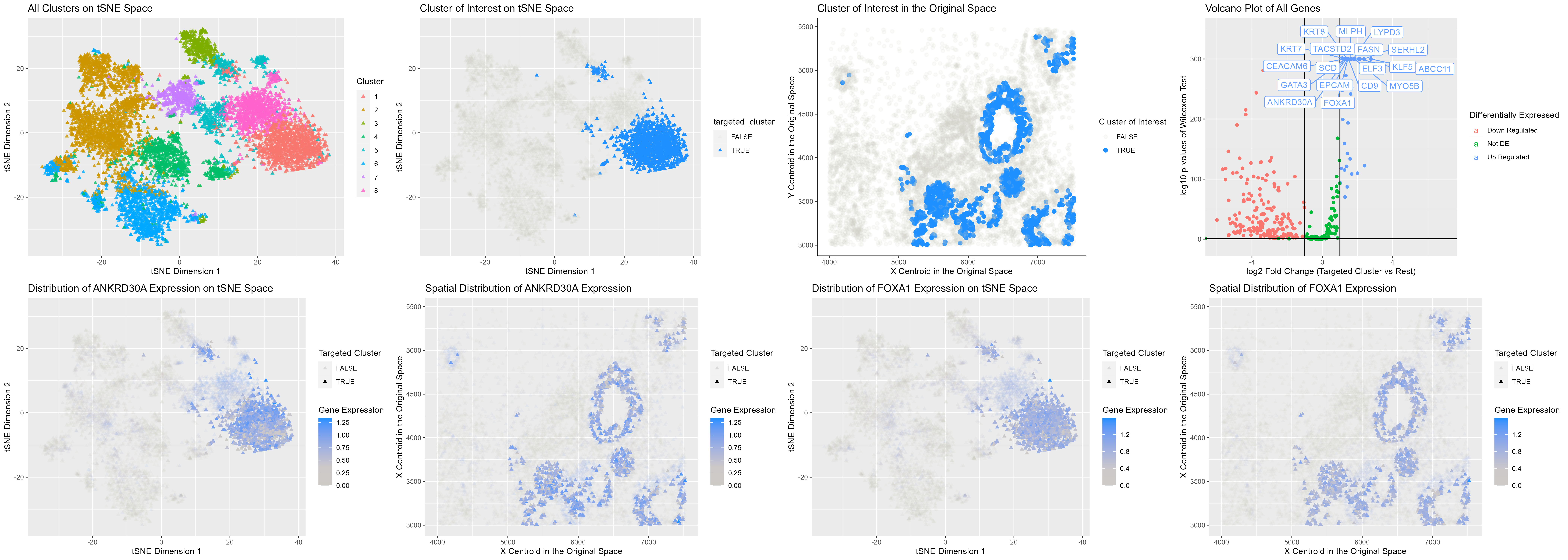
The visualization presented above comprises eight panels, all of which provide evidence to support the hypothesis that cluster 1 corresponds to breast glandular cells, a type of epithelial cell (1). The top row panels are referred to as A, B, C, and D, while the bottom row panels are labeled E, F, G, and H.
Although only eight clusters identified via Kmeans are displayed in panel A, multiple random initializations and varying cluster numbers were attempted, and the cluster assignments are consistently similar. All analyses focus on cluster 1, which appears to form hollow circular tubes in the original tissue section (panel C), indicating that these cells underlie some forms of epithelium. It is important to note that some of the cluster 1 cells are located far away from the rest in the tSNE space (panel B), which may explain why the spatial distribution of cells (panel C) is not always aggregated into clean circular openings.
After splitting the whole dataset into two groups, cluster 1 and the rest, differential expression analysis was performed. While many genes showed strong down-regulation (panel D), a dozen genes were significantly up-regulated, and these up-regulated genes are labeled. The Human Protein Atlas database indicates that many of these genes are highly expressed in breast glandular cells (2-4). The gene expression pattern of two transcription factors, ANKRD30A and FOXA1, is also displayed (panels E-H), indicating that they are highly expressed in cluster 1. ANKRD30A has been reported to be a marker gene for breast epithelial cells (5-6) due to its almost exclusive expression in breast epithelium (2). While ANKRD30A is also expressed in sperm cells, the expression levels are significantly lower (2). FOXA1 is broadly expressed across all types of glandular and squamous epithelial cells (4,7); however, its expression in spermatocytes is only 1 transcript per million (TPM), indicating that cluster 1 likely consists of breast glandular epithelial cells. Other genes that are crucial for epithelial development, such as GATA3 and ESR (3,8-9), are also significantly up-regulated in cluster 1.
In conclusion, this analysis provides strong evidence to support the hypothesis that cluster 1 corresponds to breast glandular epithelial cells.
- https://www.mskcc.org/cancer-care/types/breast/anatomy-breast
- https://www.proteinatlas.org/ENSG00000148513-ANKRD30A/single+cell+type
- https://www.proteinatlas.org/ENSG00000107485-GATA3/single+cell+type/breast
- https://www.proteinatlas.org/ENSG00000129514-FOXA1/single+cell+type
- https://www.nature.com/articles/s41467-018-04334-1
- https://www.sciencedirect.com/science/article/pii/S1084952121000549#tbl0010\
- https://www.ncbi.nlm.nih.gov/pmc/articles/PMC8533709/
- https://www.ncbi.nlm.nih.gov/pmc/articles/PMC2983489/
- https://www.ncbi.nlm.nih.gov/pmc/articles/PMC3991431/
Code took inspiration from https://biocorecrg.github.io/CRG_RIntroduction/volcano-plots.html
Code
library(ggplot2)
library(Rtsne)
library(gridExtra)
library(ggrepel)


## Read in data
data <- read.csv("squirtle.csv.gz")
posn <- data[,2:3]
gexp <- data[,5:ncol(data)]
rownames(posn) <- rownames(gexp) <- data$X

## Filter out all cells with no genes
count <- rowSums(gexp)
valid<- count > 0
posn <- posn[valid,]
gexp <- gexp[valid,]

## Log-transform with pseudo-count
totgexp <- rowSums(gexp)
gexp <- gexp/totgexp
gexp <- gexp*median(totgexp)
gexp <- log10(gexp+1)

## K-means
set.seed(0)
com <- kmeans(gexp, centers=8)
clusters <- as.factor(com$cluster) ## for categorical

## Focus on cluster #1
cluster_of_interest <- 1
targeted_cluster    <- clusters == cluster_of_interest

## Visualize cluster of interest in original space
data_clus <- cbind(posn, gexp, targeted_cluster)
p1 <- ggplot(data=data_clus,
       aes(x=x_centroid,
           y=y_centroid)) +
  geom_point(aes(color=targeted_cluster, alpha=targeted_cluster),
             shape =19,
             stroke=1) +
  scale_color_manual(values=c("#CDCDC1", "#1E90FF")) +
  theme_classic() +
  labs(x="X Centroid in the Original Space",
       y="Y Centroid in the Original Space",
       title="Cluster of Interest in the Original Space",
       color="Cluster of Interest", alpha="Cluster of Interest")

## Subset out cluster of interest vs others
target.cells <- which(com$cluster == cluster_of_interest)
others.cells <- which(com$cluster != cluster_of_interest)

## Test for differential expression
## Compute p-vals and log2 Fold Change
genes <- colnames(gexp)
pvs <- sapply(genes, function(g) {
  a <- gexp[target.cells, g]
  b <- gexp[others.cells, g]
  wilcox.test(a,b,alternative="two.sided")$p.val
})
log2fc <- sapply(genes, function(g) {
  a <- gexp[target.cells, g]
  b <- gexp[others.cells, g]
  log2(mean(a)/mean(b))
})

## Categorize points into classes, fix points with loss of precision
volcano_df <- data.frame(pvs, log2fc)
volcano_df$deg_status <- "Not DE"
volcano_df$deg_status[volcano_df$log2fc > 1  & volcano_df$pvs < 0.05] <- "Up Regulated"
volcano_df$deg_status[volcano_df$log2fc < -1 & volcano_df$pvs < 0.05] <- "Down Regulated"
volcano_df$display_name <- NA
volcano_df$display_name[volcano_df$log2fc > 1  & -log10(volcano_df$pvs) > 290] <-
  rownames(volcano_df)[volcano_df$log2fc > 1  & -log10(volcano_df$pvs) > 290]
volcano_df$pvs[volcano_df$pvs == 0] <- 1e-300

## Inspired by https://biocorecrg.github.io/CRG_RIntroduction/volcano-plots.html
## Volcano Plot
p2 <- ggplot(volcano_df,
       aes(y=-log10(pvs),
           x=log2fc,
           color=deg_status)) +
  geom_point() +
  geom_vline(xintercept=c(-1, 1)    , col="black") +
  geom_hline(yintercept=-log10(0.05), col="black") +
  ggrepel::geom_label_repel(label=volcano_df$display_name, max.overlaps=Inf) +
  xlim(-6, 7) +
  ylim(-10, 350) +
  labs(x="log2 Fold Change (Targeted Cluster vs Rest)",
      y="-log10 p-values of Wilcoxon Test",
      title="Volcano Plot of All Genes",
      color="Differentially Expressed")


# For reproducibility.
set.seed(0)
emb1 <- Rtsne(gexp)


# Plot cells on a tSNE embedded space, color cells by cluster assignment
all_cluster_tsne <- data.frame(emb1$Y, clus=clusters)
p3 <- ggplot(all_cluster_tsne,
       aes(x=X1, y=X2, col=clus)) +
  geom_point(alpha=0.8, shape=17) +
  labs(x="tSNE Dimension 1",
       y="tSNE Dimension 2",
       title="All Clusters on tSNE Space",
       color="Cluster")

# Plot cells on a tSNE embedded space, color cells by targeted cluster vs rest
targeted_cluster_vs_rest_tsne <- data.frame(emb1$Y, clus=data_clus)
p4 <- ggplot(targeted_cluster_vs_rest_tsne,
       aes(x=X1,
           y=X2,
           col=targeted_cluster,
           alpha=targeted_cluster)) +
  geom_point(shape=17) +
  labs(x="tSNE Dimension 1",
       y="tSNE Dimension 2",
       title="Cluster of Interest on tSNE Space") +
  scale_color_manual(values=c("#CDCDC1", "#1E90FF"))


# Plot cells on a tSNE embedded space, color cells by ANKRD30A
ANKRD30A_tsne <- data.frame(emb1$Y, gene_expr=gexp["ANKRD30A"], targeted_cluster=targeted_cluster)
colnames(ANKRD30A_tsne) <- c("X1", "X2", "gene_expr", "targeted_cluster")
p5 <- ggplot(ANKRD30A_tsne, aes(x=X1, y=X2, col=gene_expr, alpha=targeted_cluster)) +
  geom_point(shape=17) +
  scale_color_gradient2(low="#CDCDC1", high="#1E90FF", mid="#CDC9C9", midpoint=mean(gexp$ANKRD30A)) +
  labs(x="tSNE Dimension 1",
       y="tSNE Dimension 2",
       title="Distribution of ANKRD30A Expression on tSNE Space",
       color="Gene Expression",
       alpha="Targeted Cluster")

# Plot cells on a tSNE embedded space, color cells by FOXA1
FOXA1_tsne <- data.frame(emb1$Y, gene_expr=gexp["FOXA1"], targeted_cluster=targeted_cluster)
colnames(FOXA1_tsne) <- c("X1", "X2", "gene_expr", "targeted_cluster")
p6 <- ggplot(FOXA1_tsne, aes(x=X1, y=X2, col=gene_expr, alpha=targeted_cluster)) +
  geom_point(shape=17) +
  scale_color_gradient2(low="#CDCDC1", high="#1E90FF", mid="#CDC9C9", midpoint=mean(gexp$FOXA1)) +
  labs(x="tSNE Dimension 1",
       y="tSNE Dimension 2",
       title="Distribution of FOXA1 Expression on tSNE Space",
       color="Gene Expression",
       alpha="Targeted Cluster")


# Plot cells on the original space, color cells by ANKRD30A
ANKRD30A_original <- data.frame(posn, gene_expr=gexp["ANKRD30A"], targeted_cluster=targeted_cluster)
colnames(ANKRD30A_original) <- c("X1", "X2", "gene_expr", "targeted_cluster")
p7 <- ggplot(ANKRD30A_original, aes(x=X1, y=X2, col=gene_expr, alpha=targeted_cluster)) +
  geom_point(shape=17) +
  scale_color_gradient2(low="#CDCDC1", high="#1E90FF", mid="#CDC9C9", midpoint=mean(gexp$ANKRD30A)) +
  labs(x="X Centroid in the Original Space",
       y="X Centroid in the Original Space",
       title="Spatial Distribution of ANKRD30A Expression",
       color="Gene Expression",
       alpha="Targeted Cluster")


# Plot cells on the original space, color cells by FOXA1
FOXA1_original <- data.frame(posn, gene_expr=gexp["FOXA1"], targeted_cluster=targeted_cluster)
colnames(FOXA1_original) <- c("X1", "X2", "gene_expr", "targeted_cluster")
p8 <- ggplot(FOXA1_original, aes(x=X1, y=X2, col=gene_expr, alpha=targeted_cluster)) +
  geom_point(shape=17) +
  scale_color_gradient2(low="#CDCDC1", high="#1E90FF", mid="#CDC9C9", midpoint=mean(gexp$FOXA1)) +
  labs(x="X Centroid in the Original Space",
       y="X Centroid in the Original Space",
       title="Spatial Distribution of FOXA1 Expression",
       color="Gene Expression",
       alpha="Targeted Cluster")


g <- arrangeGrob(p3,p4,p1,p2,p5,p7,p6,p8,
                 layout_matrix=rbind(c(1,2,3,4),c(5,6,7,8))) #generates g
ggsave(file="hw5_yyang117.png",
       g,
       height=10,
       width=28,
) #saves g
