Validation of cell type clustering via differential gene expression

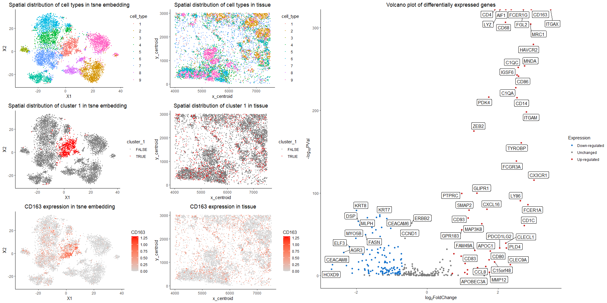
The purpose of this visualization to present the usage of differential gene expression to validate cell type identification in k-means and tsne analysis of the dataset. The quantitative data of gene expression matrix is preprocessed by removing cells with total gene counts below 10, normalized by total gene counts, and log-scaled. In the first row of the left panel, identified nine cell clusters are visualized with different color hues encoding different cell types in both tsne space and tissue sample space. I choose to run for 9 clusters, because it is relatively optimal in discerning different clusters visually without further dividing out one cluster. The most differentially expressed genes are computed in each cluster, and the rationale of choosing nine clusters is further validated based on literature search. The nine clusters all have distinct profiles for top differentially expressed genes, with the typical biomarkers of breast epithelial cells, grandular cells, T cells, macrophage, B cells, etc. Specifically, here I focus on cluster 1, and argue that it is the macrophage population. The second row of the left panel presents the position of cluster 1 in tsne space and tissue space. It forms a coherent cluster in the embedding space, while scatters through in real sample space, which agrees to the physiology of macrophages being freely floating in tissue space and migrating throughout the tumor site. From the right panel of the volcano plot, the genes with more than two fold expression change and having a p value < 0.05 are marked. Among the up-regulated genes, CD163, CD68, CD14, CD80, CD86 are all represented markers for the macrophage population. CD163 is a macrophage-specific marker and is generally not expressed in cell types other than monocytes/macrophages [1]. It is also used as a surrogate marker for macrophage phenotype in breast cancer cells[2]. CD68 is mainly localized in the membrane and cytoplasm of macrophages, while high CD68 expression has been found in 157 cases (72.4%) of breast cancer patients[3]. CD14 is made mostly by macrophages as part of the innate immune system to detect bacteria in the body[4]. CD80 is a prevalent biomarker for M1 macrophage that helps produce pro-inflammatory cytokines[5]. CD86 is also primarily expressed on dendritic cells, and other major immune population[6]. Thus, collectively speaking, it is the most likely that cluster 1 is the macrophage population. In the third row of the left panel, I choose to visualize the quantitative data of CD163 expression on tsne plot and tissue space. Because CD163 has a small p value as well as a high fold change. We could see that CD163 expression pattern corresponds well to cluster 1 distrbution. Thus, the claim that cluster 1 is the macrophage population is validated.

Reference.

[1]https://www.proteinatlas.org/ENSG00000177575-CD163 [2]Garvin, Stina et al. “Tumor cell expression of CD163 is associated to postoperative radiotherapy and poor prognosis in patients with breast cancer treated with breast-conserving surgery.” Journal of cancer research and clinical oncology vol. 144,7 (2018): 1253-1263. doi:10.1007/s00432-018-2646-0 [3]Yuan, J., He, H., Chen, C. et al. Combined high expression of CD47 and CD68 is a novel prognostic factor for breast cancer patients. Cancer Cell Int 19, 238 (2019). https://doi.org/10.1186/s12935-019-0957-0 [4]https://en.wikipedia.org/wiki/CD14#:~:text=CD14%20(cluster%20of%20differentiation%2014,associated%20molecular%20pattern%20(PAMP) [5]Bertani, Francesca R et al. “Classification of M1/M2-polarized human macrophages by label-free hyperspectral reflectance confocal microscopy and multivariate analysis.” Scientific reports vol. 7,1 8965. 21 Aug. 2017, doi:10.1038/s41598-017-08121-8 [6]https://www.sciencedirect.com/topics/biochemistry-genetics-and-molecular-biology/cd86#:~:text=CD86%20is%20constitutively%20expressed%20on,of%20a%20variety%20of%20cytokines.

Code modified from in-class notes.

Please note that the final output has adjusted canvas size for importing.

Code

library(Rtsne)
library(ggplot2)
library(gridExtra)
library(ggrepel)

data <- read.csv('genomic-data-visualization-2023/data/charmander.csv.gz', row.names = 1)
## pull out gene expression
pos <- data[,1:2]
gexp <- data[, 4:ncol(data)]

good.cells <- rownames(gexp)[rowSums(gexp) > 10]
pos <- pos[good.cells,]
gexp <- gexp[good.cells,]

totgexp <- rowSums(gexp)
mat <- gexp/totgexp
mat <- mat*median(totgexp)
mat <- log10(mat + 1)

#perform tsne
set.seed(0) ## for reproducibility
emb <- Rtsne::Rtsne(mat)
com <- kmeans(mat, centers=9) #choose 9 centers as tuned visually from tsne plot

#plot embedding
df <- data.frame(pos, emb$Y, cell_type=as.factor(com$cluster),cluster_1 = (com$cluster == 1))
#plot embedding in tsne space
p1 <- ggplot(df, aes(x = X1, y = X2, col=cell_type)) + 
  geom_point(size = 0.1) +
  ggtitle("Spatial distribution of cell types in tsne embedding")+
  theme_classic()+
  theme(plot.title = element_text(hjust = 0.5))
p1
#plot embedding in tissue space
p2 <- ggplot(df, aes(x = x_centroid, y = y_centroid, col=cell_type)) + 
  geom_point(size = 0.1) + 
  ggtitle("Spatial distribution of cell types in tissue")+
  theme_classic()+
  theme(plot.title = element_text(hjust = 0.5))
p2
#plot embedding in tsne space
p3 <- ggplot(df, aes(x = X1, y = X2, col=cluster_1)) + 
  geom_point(size = 0.1) +
  ggtitle("Spatial distribution of cluster 1 in tsne embedding")+
  scale_color_manual(values = c("gray50", "red")) +
  theme_classic()+
  theme(plot.title = element_text(hjust = 0.5))
p3
#plot embedding in tissue space
p4 <- ggplot(df, aes(x = x_centroid, y = y_centroid, col=cluster_1)) + 
  geom_point(size = 0.1) + 
  ggtitle("Spatial distribution of cluster 1 in tissue")+
  scale_color_manual(values = c("gray50", "red")) +
  theme_classic()+
  theme(plot.title = element_text(hjust = 0.5))
p4

## pick a cluster
#cluster 1: CD163, CD4, CD68, CD86, CD14/macrophage
## pick a cluster
cluster_num = 1
cluster.of.interest <- names(which(com$cluster == cluster_num))
cluster.other <- names(which(com$cluster != cluster_num))
## loop through my genes and test each one
genes <- colnames(mat)
pvs <- sapply(genes, function(g) {
  a <- mat[cluster.of.interest, g]
  b <- mat[cluster.other, g]
  wilcox.test(a,b,alternative="two.sided")$p.val
})
names(which(pvs < 1e-8))
head(sort(pvs), n=20)

### calculate a fold change
log2fc <- sapply(genes, function(g) {
  a <- mat[cluster.of.interest, g]
  b <- mat[cluster.other, g]
  log2(mean(a)/mean(b))
})


## volcano plot
deg <- data.frame(pvs, log2fc)
Expression <- apply(deg, 1, function(g) {
  if (g[2] >= log(2) & g[1] <= 0.05) {
    out = "Up-regulated"
  } else if (g[2] <= -log(2) & g[1] <= 0.05) {
    out = "Down-regulated"
  } else {
    out = "Unchanged"
  }
  out
})
deg <- cbind(deg, Expression)

options(repr.plot.width = 8, repr.plot.height =4)
p5 <- ggplot(deg, aes(y=-log10(pvs), x=log2fc)) + 
  geom_point(aes(color = Expression)) +
  xlab(expression("log"[2]*"FoldChange")) + 
  ylab(expression("-log"[10]*"PVal")) +
  scale_color_manual(values = c("dodgerblue3", "gray50", "firebrick3")) +
  guides(colour = guide_legend(override.aes = list(size=1.5))) +
  ggrepel::geom_label_repel(label=rownames(deg), force = 2)+
  ggtitle("Volcano plot of differentially expressed genes")+
  theme_classic()+
  theme(plot.title = element_text(hjust = 0.5))
p5

#visualize CD163, since it is high in fold change with very small p value

df <- cbind(df,CD163 = mat$CD163)
#plot embedding in tsne space
p6 <- ggplot(df, aes(x = X1, y = X2, col = CD163)) + 
  geom_point(size = 0.1) +
  ggtitle("CD163 expression in tsne embedding")+
  theme_classic()+
  theme(plot.title = element_text(hjust = 0.5))+
  scale_color_gradient(low = 'lightgrey', high='red') 
p6
#plot embedding in tissue space
p7 <- ggplot(df, aes(x = x_centroid, y = y_centroid, col=CD163)) + 
  geom_point(size = 0.1) + 
  ggtitle("CD163 expression in tissue")+
  theme_classic()+
  theme(plot.title = element_text(hjust = 0.5))+
  scale_color_gradient(low = 'lightgrey', high='red')
p7

g1 <- grid.arrange(p1, p2, p3, p4,p6,p7,ncol=2)
g2<- grid.arrange(g1, p5,ncol=2)
g2
#source used
#https://samdsblog.netlify.app/post/visualizing-volcano-plots-in-r/