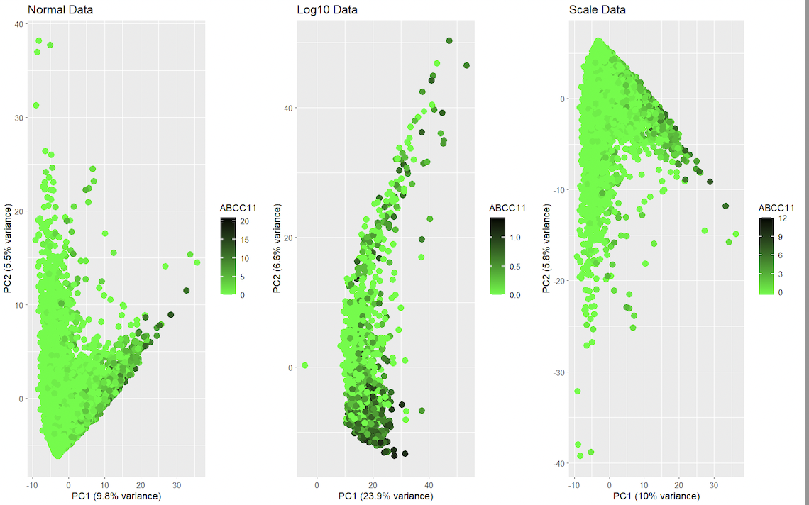
1. Should I normalize and/or transform the gene expression data (e.g. log and/or scale) prior to dimensionality reduction?

It is recommended to normalize the data with scale to help take into consideration the differences in variability and scale in the genes, for example making sure if some genes have large range, it doesn’t affect the final PCA score. With log it helps reduce sudden changes in distributions.

2. Should I perform non-linear dimensionality reduction on genes or PCs?

Ideally uncover non-linear relationships among genes, using t-SNE on the gene expression data.

3. If I perform non-linear dimensionality reduction on PCs, how many PCs should I use?

The amount of PC’s can be visualized with a variance plot, showing the cumulative explained variance versus the numbers of PCs used. By plotting the cumulative variance in this dataset and establishing for example 85% desired variance in this dataset, the number of PCs is either 2 or 3. In the case of this code I will be using 2.

4. What genes (or other cell features such as area or total genes detected) are driving my reduced dimensional components?

The genes used are ZEB1 and ZEB2, and the other cell features driving the reduced dimensional component is area.

5. Write a description describing your data visualization using vocabulary terms from Lesson 1.

This data visualization renders the first two principal components for both genes ZEB1 and ZEB2 side by side for comparison from the spatial transcriptomics dataset. It uses categorical data with geometric primitives such as points for encoding. It displays visual changes using positions hue in color, also uses similarity in color and proximity in data points as the gestalt principles.

Code

library(ggplot2) library(gridExtra)

#Load data df <- read.csv(‘/Users/YourUsername/Desktop/data/squirtle.csv.gz’, row.names = 1)

#log #df[, c(“x_centroid”, “y_centroid”, “area”)] <- log(df[, c(“x_centroid”, “y_centroid”, “area”)])

#scale df[, c(“x_centroid”, “y_centroid”, “area”)] <- scale(df[, c(“x_centroid”, “y_centroid”, “area”)])

#Perform PCA pca <- prcomp(df[, c(“x_centroid”, “y_centroid”, “area”)], scale = TRUE)

#get number of PCAs cumulative_var <- cumsum(pca$sdev^2/sum(pca$sdev^2))

plot(cumulative_var, xlab = “Number of Principal Components”, ylab = “Cumulative Proportion of Variance Explained”, type = “b”)

desired_var <- 0.85 # for example, let’s say we want to explain 85% of the variance num_pcs <- which(cumulative_var > desired_var)[1]

num_pcs

df$PC1 <- pca$x[, 1] df$PC2 <- pca$x[, 2]

#Plot first two principal components for ZEB1 p1 <- ggplot(df, aes(x = PC1, y = PC2, color = ZEB1)) + geom_point(size = 3) + scale_color_gradient(name = “ZEB1”, low = “green”, high = “red”) + ggtitle(“PCA of Spatial Transcriptomics Data for ZEB1”) + xlab(paste0(“PC1 (“, round(pca$sdev[1]^2/sum(pca$sdev^2)100, 1), “% variance)”)) + ylab(paste0(“PC2 (“, round(pca$sdev[2]^2/sum(pca$sdev^2)100, 1), “% variance)”))

#Plot first two principal components for ZEB2 p2 <- ggplot(df, aes(x = PC1, y = PC2, color = ZEB2)) + geom_point(size = 3) + scale_color_gradient(name = “ZEB2”, low = “green”, high = “red”) + ggtitle(“PCA of Spatial Transcriptomics Data for ZEB2”) + xlab(paste0(“PC1 (“, round(pca$sdev[1]^2/sum(pca$sdev^2)100, 1), “% variance)”)) + ylab(paste0(“PC2 (“, round(pca$sdev[2]^2/sum(pca$sdev^2)100, 1), “% variance)”))

#Combine the two plots into one image grid.arrange(p1, p2, ncol = 2)

External resources

Hayden, L. (2018, August 09). R PCA tutorial (principal component analysis). Retrieved February 6, 2023, from https://www.datacamp.com/tutorial/pca-analysis-r Pramoditha, R. (2022, April 25). How to select the best number of Principal Components for the Dataset. Retrieved February 6, 2023, from https://towardsdatascience.com/how-to-select-the-best-number-of-principal-components-for-the-dataset-287e64b14c6d