Definition of cell type on breast tissue

HW 5
Definition of cell type on breast tissue:
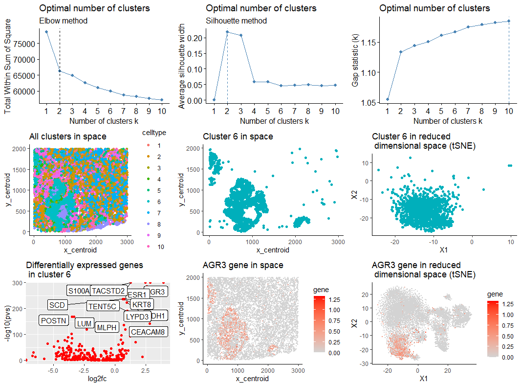
Given the differential gene expression analysis, the cell type equivalent to cluster 6 in the data file is most likely a breast glandular cell. Having identified the overexpressed genes in this cluster, the following were searched in The Human Protein Atlas under Breast tissue and ranked by correlation with each cell type (e.g., https://www.proteinatlas.org/ENSG00000121966-CXCR4/tissue+cell+type/breast). Based on the results, the higher correlation was with Breast Glandular cell 1, as shown in the Sum row at the following table.
1
2
3
4
5
6
7
8
9
10
11
12
	    Breast glandular cells_2	Breast glandular cell 1	T-cell	Breast myoepithelial cell	  Plasma cell
AGR3	      0.788	                    0.62                	0.5	        0.499	                  0.468
ESR1	      0.69	                    0.609	                0.47	      0.58                   	0.379
KRT8	      0.645                   	0.741                	0.597     	0.688	                  0.517
LYPD3	      0.62	                    0.754               	0.552	      0.671	                  0.557
TENT5C	    0.6	                      0.58	                0.743     	0.604	                  0.802
TACSTD2	    0.55	                    0.7	                  0.5	        0.716	                  0.467
S100A14	    0.68	                    0.81	                0.52	      0.62	                  0.597
SERPINA3	  0.34	                    0.589	                0.016     	0.182	                  0.349
CEACAM6	    0.51	                    0.48	                0.44	      0.45	                  0.42

Sum	        5.423	                    5.883	                4.338	      5.01	                  4.556
Commented code:
1
2
3
4
5
6
7
8
9
10
11
12
13
14
15
16
17
18
19
20
21
22
23
24
25
26
27
28
29
30
31
32
33
34
35
36
37
38
39
40
41
42
43
44
45
46
47
48
49
50
51
52
53
54
55
56
57
58
59
60
61
62
63
64
65
66
67
68
69
70
71
72
73
74
75
76
77
78
79
80
81
82
83
84
85
86
87
88
89
90
91
92
93
94
95
96
97
98
99
100
101
102
103
104
105
106
107
108
109
110
111
112
113
114
115
116
117
118
119
120
121
122
123
124
125


data <- read.csv('pikachu.csv.gz', row.names=1)
pos <- data[,1:2] # x centroid and y centroid
gexp <- data[, 4:ncol(data)] # gene expression

good.cells <- rownames(gexp)[rowSums(gexp) > 10] # get rid of 0s
pos <- pos[good.cells,]
gexp <- gexp[good.cells,]


totgexp <- rowSums(gexp) # total genes expressed by each cell
mat <- gexp/totgexp # Normalize per max expression
mat <- mat*median(totgexp) #
mat <- log10(mat + 1) # scale

set.seed(1)
# Dimension reduction and clustering
emb <- Rtsne::Rtsne(mat) # :: directly access a member of a package that is internal

# Define number of clusters

library(factoextra)
library(NbClust)
library(cluster)
library(ggrepel) ## install.packages("ggrepel")

# Elbow method
p01<-fviz_nbclust(mat, kmeans, method = "wss") +
  geom_vline(xintercept = 2, linetype = 2)+
  labs(subtitle = "Elbow method")
# Silhouette method
p02 <-fviz_nbclust(mat, kmeans, method = "silhouette")+
  labs(subtitle = "Silhouette method")

# gap statistic
set.seed(123)
gap_stat <- clusGap(mat, FUN = kmeans, nstart = 25,
                    K.max = 10, B = 50)


p03<-fviz_gap_stat


library(gridExtra)
library(grid)
library(ggplot2)
library(lattice)
grid.arrange(p01,p02,p03,nrow=1,top=textGrob("Number of clusters",gp=gpar(fontsize=20)),
             right =textGrob("Gap statistic method",x=0.0001,y=0.9))

# Comparing the 3 methods, the number of clusters should be 2. Since number of diff
# expressed genes in cluster 2 is too large for 2 clusters, let's work with 10.
########################################################################
com <- kmeans(mat, centers=10) ##

## plot my clusterings in embedding and tissue space
library(ggplot2)
df_nonReduced <- data.frame(pos, celltype=as.factor(com$cluster))
df_nonReduced_c2 <- subset(df_nonReduced,celltype==6)

df <- data.frame(pos, emb$Y, celltype=as.factor(com$cluster))
df2 <- subset(df, celltype == 6)


head(df2)
p_orig <- ggplot(df, aes(x = x_centroid, y = y_centroid, col=celltype)) +
  geom_point(size=1.5) + theme_classic()+ ggtitle("All clusters in space")

p1 <- ggplot(df_nonReduced_c2, aes(x = x_centroid, y = y_centroid)) +
  geom_point(size=1.5,color = "#00AFBB") + theme_classic()+ ggtitle("Cluster 6 in space")

p2 <- ggplot(df2, aes(x = X1, y = X2)) + geom_point(size = 1.5,color = "#00AFBB") +
  scale_colour_brewer('My groups', palette = 'Set2') +
  theme_classic()+ ggtitle("Cluster 6 in reduced \n dimensional space (tSNE)")


## pick a cluster
cluster.of.interest <- names(which(com$cluster == 6))
cluster.other <- names(which(com$cluster != 6))
## loop through my genes and test each one
genes <- colnames(mat)
# Find differentially expressed genes (comparing clusters)
# Wilcox text determine if two or more sets of pairs are different from one another in
# a statistically significant manner.
pvs <- sapply(genes, function(g) {
  a <- mat[cluster.of.interest, g]
  b <- mat[cluster.other, g]
  wilcox.test(a,b,alternative="two.sided")$p.val
})

table(pvs < 0.05)
pvs[names(which(pvs < 0.05))]

head(sort(pvs), n=20)

# Visualize differentially expressed genes
### calculate a fold change
log2fc <- sapply(genes, function(g) {
  a <- mat[cluster.of.interest, g]
  b <- mat[cluster.other, g]
  log2(mean(a)/mean(b))
})

# df_genes <- data.frame(pvs, log2fc)
# ggplot(df_genes, aes(y=-log10(pvs), x=log2fc)) + geom_point()

p_genes <- ggplot(df_genes, aes(y=-log10(pvs), x=log2fc)) + geom_point(color = "red") +
  ggrepel::geom_label_repel(label=rownames(df_genes)) + ggtitle("Differentially expressed genes \n in cluster 6")

## Select a gene among the top differentially expressed in cluster 6.
g <- 'AGR3'
df_g <- data.frame(pos, emb$Y, gene=mat[,g])
head(df)
p_Ag3 <- ggplot(df, aes(x = x_centroid, y = y_centroid, col=gene)) +
  geom_point(size = 0.1) + theme_classic() + scale_color_continuous(low='lightgrey', high='red')+
  ggtitle("AGR3 gene in space")

p_Ag3_tSNE <- ggplot(df, aes(x = X1, y = X2, col=gene)) + geom_point(size = 0.1) +
  theme_classic() + scale_color_continuous(low='lightgrey', high='red')+
  ggtitle("AGR3 gene in reduced \n dimensional space (tSNE)")


# Final visualization
grid.arrange(p01,p02,p03,p_orig,p1,p2,p_genes,p_Ag3,p_Ag3_tSNE,nrow=3,ncol=3)
References
https://www.datanovia.com/en/lessons/determining-the-optimal-number-of-clusters-3-must-know-methods/#computing-the-number-of-clusters-using-r https://predictivehacks.com/how-to-determine-the-number-of-clusters-of-k-means-in-r/#google_vignette https://www.proteinatlas.org/