Cell Type Exploration of Charmander Data Set

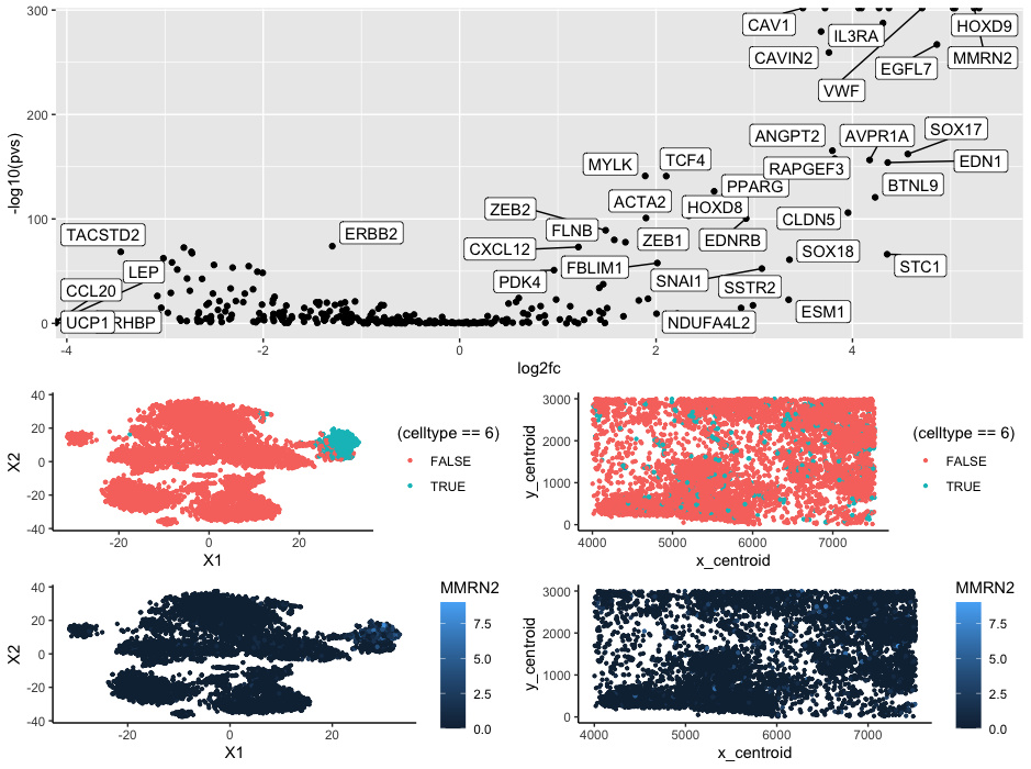
The cluster appears to be endothelial cells that make up adipose tissue. When looking at the Wilcox vs log2fc graph three of most significantly upregulated genes are CAV1, VWF, and MMRN2. Using ProteinAtlas (https://www.proteinatlas.org/), we can see that all three of these genes correspond to endothelial/adipose tissue clusters which lead me to make the conclusion that this is what the cluster is. Additionally when looking at the cluster in space we can see that the cluster is spread out but located between other cells or acts as bridges between spatial structures which is something that we could expect out of a connective tissue such as adipose tissue.
1
2
3
4
5
6
7
8
9
10
11
12
13
14
15
16
17
18
19
20
21
22
23
24
25
26
27
28
29
30
31
32
33
34
35
36
37
38
39
40
41
42
43
44
45
46
47
48
49
50
51
52
53
54
55
56
57
58
59
60
61
62
63
64
65
66
67
68
69
70
71
72
73
74
75
76
77
78
79
80
81
82
83
84
85
86
87
library(Rtsne)
library(tidyverse)
library(ggokabeito)
library(gganimate)
library(gifski)
library(ggrepel)
library(gridExtra)

##Most code adapted from Prof. Fan "code-02-13-2023" code unless otherwise noted

data <- read.csv('Downloads/charmander.csv.gz',row.names=1)

##Capture gene expression
pos <- data[,1:2]
gexp <- data[,4:ncol(data)]

##Normalize
good.cells <-rownames(gexp)[rowSums(gexp) > 10]
pos <- pos[good.cells,]
gexp <- gexp[good.cells,]

totgexp <- rowSums(gexp)
mat <- gexp/totgexp
mat <- mat*median(totgexp)
max <- log10(mat+1)

#Get only unique values because tsne gets mad
matUnique <- unique(mat)

#find principal component number that makes sense (taken from class)
pcs <- prcomp(matUnique)
par(mfrow=c(1,1))
plot(1:10,pcs$sdev[1:10],type='l')

#Using above graph, used only six principal components
set.seed(8)
pcsIm <- pcs$x[,1:6]
emb <- Rtsne::Rtsne(pcsIm)

#Taken from Prof. Fan/I think Ryan in class on how to decide how many clusters to pick (10)
results <- do.call(rbind, lapply(seq_len(15), function(k) {
  out <- kmeans(matUnique,centers=k, iter.max=50)
  c(out$tot.withinss,out$betweenss)
}))
plot(seq_len(15),results[,1], main='tot.withinss')
plot(seq_len(15),results[,2], main='tot.betweenss')

com <- kmeans(matUnique, centers=10)

df <- data.frame(pos, emb$Y, celltype=as.factor(com$cluster))
head(df)
p1 <- ggplot(df, aes(x = X1, y = X2, col=(celltype==6))) + geom_point(size = 0.8) +
  theme_classic()
p2 <- ggplot(df, aes(x = x_centroid, y = y_centroid, col=(celltype==6))) +
  geom_point(size = 0.8) + theme_classic()

## pick a cluster
cluster.of.interest <- names(which(com$cluster == 6))
cluster.other <- names(which(com$cluster != 6))

genes <- colnames(matUnique)
pvs <- sapply(genes, function(g) {
  a <- matUnique[cluster.of.interest, g]
  b <- matUnique[cluster.other, g]
  wilcox.test(a,b,alternative="two.sided")$p.val
})

log2fc <- sapply(genes, function(g) {
  a <- matUnique[cluster.of.interest, g]
  b <- matUnique[cluster.other, g]
  log2(mean(a)/mean(b))
})

df2 <- data.frame(pvs, log2fc)

p3 <- ggplot(df2, aes(y=-log10(pvs), x=log2fc)) + geom_point() +
  ggrepel::geom_label_repel(label=rownames(df2))

names(which(pvs < 1e-323))

df3 <- data.frame(pos, emb$Y, gexp)
p4 <- ggplot(df3, aes(x = X1, y = X2, col=MMRN2)) + geom_point(size = 0.8) +
  theme_classic()
p5 <- ggplot(df3, aes(x = x_centroid, y = y_centroid, col=MMRN2)) +
  geom_point(size = 0.8) + theme_classic()

grid.arrange(p3,grid.arrange(nrow=2,ncol=2,p1,p2,p4,p5))