How STcompare works • STcompare

This article walks through what compareSpatial() computes for one gene, step by step, with small examples from the data that ship with the package:

Matched pixels: the two samples are compared pixel by pixel.
Pearson’s correlation, and why its usual p-value fails for spatial data.
Spatially autocorrelated surrogates with the gene’s own values, which give a valid null distribution.
Sequential permutation p-values that stop early when the answer is clear.
Both directions, one p-value per gene and the adjustment for multiple testing.
Rarely detected genes: why the surrogates take the gene’s own values.
Spatial similarity: the expression levels at matched pixels.

library(STcompare)
library(SpatialExperiment)
library(ggplot2)
library(patchwork)
data(speKidney)
data(simRanPatternRasts)

Matched pixels

STcompare compares the same locations in two samples. After the tissues are aligned, both samples are rasterized together onto one grid of pixels, here hexagons, so that a pixel name refers to the same location in both:

rast <- SEraster::rasterizeGeneExpression(speKidney, assay_name = "counts",
                                          resolution = 0.2, fun = "mean",
                                          square = FALSE)
shared <- intersect(colnames(rast$A), colnames(rast$B))
length(shared)
#> [1] 273

For a gene, the comparison uses two vectors over the shared pixels: its values in the first sample, x, and in the second, y.

x <- assay(rast$A, "pixelval")["Gene", shared]
y <- assay(rast$B, "pixelval")["Gene", shared]
coords <- spatialCoords(rast$A)[shared, ]

To draw maps of values on these pixels, we put them into a copy of the rasterized object and use SEraster::plotRaster():

mapValues <- function(values, title) {
  spe <- rast$A[, shared]
  assay(spe, "pixelval") <- matrix(values, nrow = 1,
                                   dimnames = list("Gene", shared))
  SEraster::plotRaster(spe, plotTitle = title, showLegend = FALSE)
}
mapValues(x, "x: A") + mapValues(y, "y: B")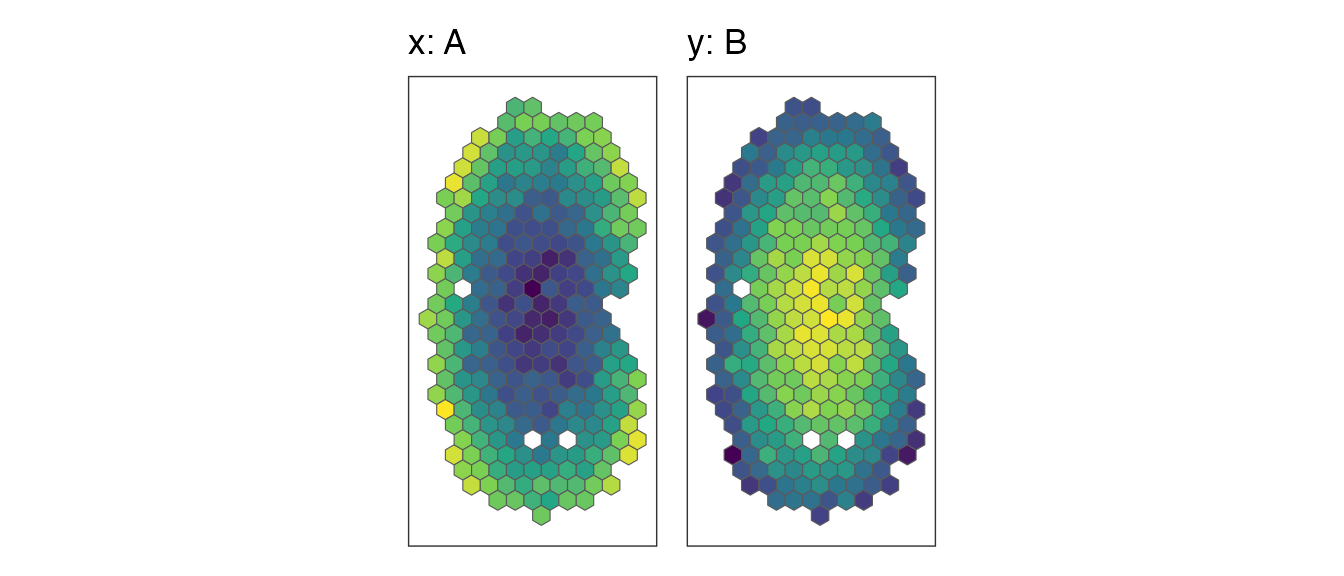

Maps of the values of Gene on the pixels shared by kidneys A and B: the two patterns are opposite.

Pearson’s correlation, and why the naive p-value fails

The statistic is Pearson’s correlation of x and y over the shared pixels:

cor(x, y)
#> [1] -0.9472813

Its usual test, cor.test(), assumes that the pixels are independent observations. In a tissue they are not: neighbouring pixels have similar values, so a smooth pattern carries far less independent information than its number of pixels suggests, and two unrelated smooth patterns often have a sizeable correlation. simRanPatternRasts holds 100 independently simulated, spatially autocorrelated patterns on one grid. The correlations of all 4950 pairs of them are spread much more widely than the correlations of independent pixels would be:

values <- lapply(simRanPatternRasts, function(s) assay(s, "pixelval")[1, ])
pairs <- utils::combn(length(values), 2)
pairR <- apply(pairs, 2, function(ij) {
  common <- intersect(names(values[[ij[1]]]), names(values[[ij[2]]]))
  c(r = cor(values[[ij[1]]][common], values[[ij[2]]][common]),
    pixels = length(common))
})
r <- pairR["r", ]
pixels <- pairR["pixels", ]
# the p-value of cor.test() for each pair
naiveP <- 2 * pt(-abs(r) * sqrt((pixels - 2) / (1 - r^2)), df = pixels - 2)
n <- median(pixels)
ggplot(data.frame(r = r), aes(r)) +
  geom_histogram(aes(y = after_stat(density)), bins = 50, fill = "grey70") +
  stat_function(fun = function(r) dnorm(r, sd = 1 / sqrt(n - 3)),
                colour = "red") +
  labs(x = "Correlation of two unrelated patterns", y = "Density") +
  theme_classic()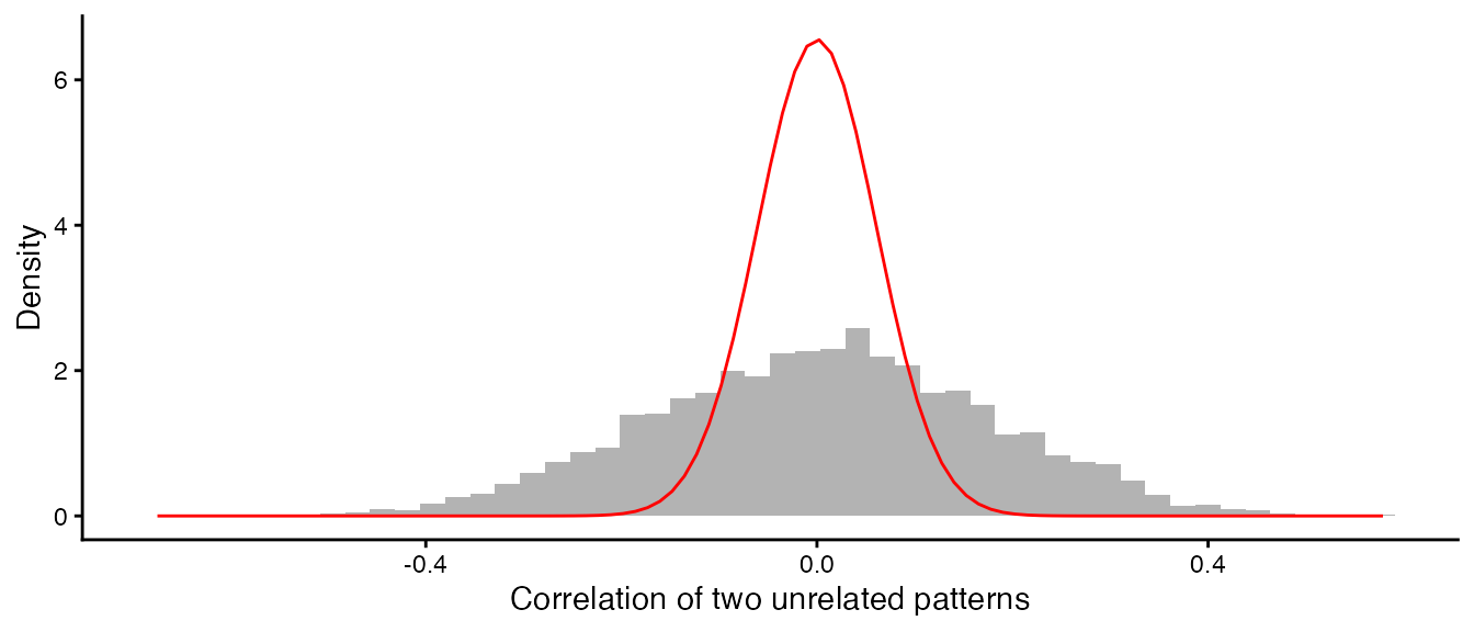

Histogram of the correlations of 4950 pairs of unrelated simulated patterns, much wider than the red curve of the correlation of independent pixels.

The red curve is the distribution of r for 273 independent pixels, with a standard deviation of 0.061; the observed standard deviation is 0.171. The patterns behave as if they had about 37 independent observations rather than 273. As a result, cor.test() gives p < 0.05 for 50% of these unrelated pairs instead of 5%. STcompare therefore builds the null distribution of r from surrogate patterns with the same spatial autocorrelation.

A null distribution that keeps the spatial autocorrelation

STcompare uses the method of Viladomat et al. (2014). To test the correlation of x with y, it generates surrogates of x: random patterns that have the same spatial autocorrelation as x, and the same values, but no relation to y. Each surrogate is made in five steps.

1. Shuffle the values of x across the pixels. This keeps the values but destroys the spatial pattern, and with it the autocorrelation.

set.seed(1)
shuffled <- x[sample.int(length(x))]

2. Smooth the shuffled values with a Gaussian kernel whose window holds a share $\delta$ of the pixels (a nearest-neighbour bandwidth). A small $\delta$ gives a rough pattern and a large one a smooth pattern. The smoother is the local-constant fit of locfit::locfit(kern = "gauss", nn = delta), evaluated on locfit’s adaptive tree, reimplemented in C++.

3. Match the variogram. The variogram $\gamma(h)$ is half the mean squared difference between the values of two pixels at distance $h$ ; it describes how fast similarity decays with distance. STcompare computes it up to the 25% quantile of the pixel distances (maxDistPrctile; with more than 1000 pixels, on a random subset of 1000 pixels, for speed), fits the variogram of x as a linear function of the variogram of the smoothed values, $\gamma_x(h) \approx \beta_0 + \beta_1 \gamma_\delta(h)$ , and forms the surrogate $\sqrt{|\beta_1|}\, x_\delta + \sqrt{|\beta_0|}\, Z$ , where $Z$ is Gaussian noise. Rescaling matches the slope of the variogram and the noise its intercept (the nugget).

4. Choose $\delta$ . Steps 2 and 3 are done for every $\delta$ of the grid (delta, by default 0.01, 0.05 and 0.1 to 0.9), and the $\delta$ whose surrogate’s variogram is closest to the variogram of x (smallest residual sum of squares), delta star, gives the surrogate.

5. Remap the values. The smoothed, rescaled surrogate has values that are close to normally distributed, whatever the distribution of x. Its values are therefore replaced by the values of x themselves, placed in the surrogate’s rank order: the pixel with the smallest surrogate value gets the smallest value of x, and so on (the amplitude adjustment of Theiler et al. 1992; surrogate = "remap", the default). The surrogate keeps the spatial arrangement of step 3 and has exactly the distribution of values of x, zeros included. Rarely detected genes shows why this matters; surrogate = "gaussian" skips this step and gives the surrogates of the legacy functions.

The legacy function viladomatCorrelation() exposes the surrogates of steps 1 to 4. With a single $\delta$ it returns the surrogate for that bandwidth, and with the same seed it starts from the same shuffle as above; step 5 is one line of R:

xyData <- cbind(x, y, coords)
grid <- c(0.01, 0.05, seq(0.1, 0.9, 0.1))
smoothed <- function(delta) {
  viladomatCorrelation(xyData, delta = delta, maxDistPrctile = 0.25,
                       nPermutations = 1, seed = 1)
}
remap <- function(surrogate, values) {
  remapped <- surrogate
  remapped[order(surrogate)] <- sort(values)
  remapped
}
deltaStar <- smoothed(grid)$deltaStar
deltaStar
#> [1] 0.2
shown <- unique(c(0.01, 0.05, deltaStar, 0.6))
gaussian <- lapply(shown, function(d) smoothed(d)$permutations[, 1])
fields <- c(list(x = x, shuffled = shuffled),
            lapply(gaussian, remap, values = x))
names(fields)[-(1:2)] <- ifelse(shown == deltaStar, "delta* ", "delta ")
names(fields)[-(1:2)] <- paste0(names(fields)[-(1:2)], shown)
wrap_plots(Map(mapValues, fields, names(fields)), nrow = 1)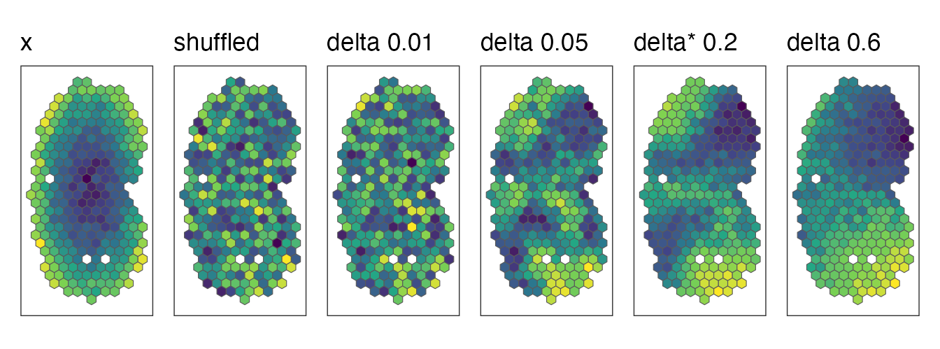

Maps of x, of its shuffled values, and of remapped surrogates smoothed with increasing bandwidths: the shuffled values have no pattern, and larger bandwidths give smoother surrogates, all with the values of x.

Every map has the same values, those of x, arranged differently: shuffled, or smoothed with increasing bandwidths.

The variograms show why delta star is 0.2 for this surrogate. Delta star is chosen in step 4, from the variograms of the smoothed, rescaled surrogates; the remapping is a monotone change of the amplitudes, which alters the variogram only a little, so the variograms of the remapped surrogates tell the same story. We compute them with a small helper, in equal distance bins up to the 25% quantile of the distances (STcompare’s own computation follows geoR::variog()):

variogram <- function(values, coords, maxDist, nBins = 12) {
  d <- as.matrix(dist(coords))
  halfSq <- outer(values, values, function(a, b) (a - b)^2 / 2)
  pair <- upper.tri(d) & d <= maxDist
  bin <- cut(d[pair], seq(0, maxDist, length.out = nBins + 1))
  v <- data.frame(distance = as.numeric(tapply(d[pair], bin, mean)),
                  semivariance = as.numeric(tapply(halfSq[pair], bin, mean)))
  v[!is.na(v$distance), ]
}
maxDist <- quantile(dist(coords), 0.25)
curves <- do.call(rbind, Map(function(v, label) {
  data.frame(variogram(v, coords, maxDist), field = label)
}, fields, names(fields)))
curves$field <- factor(curves$field, levels = names(fields))
target <- curves[curves$field == "x", ]
beforeRemap <- variogram(gaussian[[which(shown == deltaStar)]], coords, maxDist)
ggplot(curves, aes(distance, semivariance, colour = field)) +
  geom_line(linewidth = 0.8) +
  geom_line(data = beforeRemap, colour = "black", linetype = "dashed") +
  geom_point(data = target, colour = "black", size = 2) +
  coord_cartesian(ylim = c(0, 1.5 * max(target$semivariance))) +
  scale_colour_manual(values = c("black", "grey60",
                                 "#E69F00", "#56B4E9", "#009E73", "#CC79A7")) +
  labs(x = "Distance", y = "Semivariance", colour = NULL) +
  theme_classic()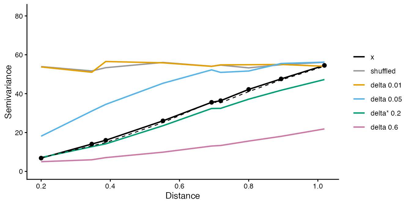

Variograms of x (black points), of the shuffled values (flat) and of the remapped surrogates: the surrogate at delta star follows the variogram of x most closely. A dashed line shows the surrogate at delta star before the remapping.

The variogram of x (black points) rises with distance: nearby pixels are similar. The shuffled values have a flat variogram. A small bandwidth leaves a rough pattern whose variogram rises too fast and flattens, a large one an over-smoothed pattern whose variogram rises too slowly, and delta star follows the variogram of x closely, before the remapping (dashed) and after it.

6. Null correlations. The correlation of each surrogate of x with y is one draw from the null distribution of r. The same is done in the other direction, with surrogates of y correlated with x. keepNulls = TRUE keeps these null correlations:

ab <- compareSpatial(rast[c("A", "B")], nPermutations = 999, nThreads = 2,
                     keepNulls = TRUE)
#> compareSpatial: 1 gene on 273 shared pixels in 0.2 s (999 permutations in total, 2 threads)
nulls <- attr(ab, "details")$Gene
ggplot(data.frame(r = c(nulls$nullX, nulls$nullY),
                  direction = rep(c("surrogates of A", "surrogates of B"),
                                  each = length(nulls$nullX))), aes(r)) +
  geom_histogram(bins = 40, fill = "grey70") +
  geom_vline(xintercept = ab$correlationCoef, colour = "red") +
  facet_wrap(~direction) +
  labs(x = "Null correlation", y = "Permutations") +
  theme_classic()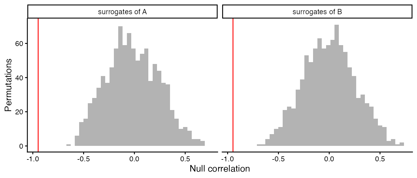

Histograms of the null correlations of the surrogates of A and of B; the observed correlation, a red line, lies far outside both.

The observed correlation of A and B (red line) lies far outside both null distributions. The nulls are wide, because unrelated smooth patterns can correlate strongly, but -0.95 is out of their reach.

Sequential p-values: stop early when the answer is clear

With $B$ permutations, the permutation p-value of a direction is $(b + 1) / (B + 1)$ , where $b$ counts the null correlations at least as extreme as the observed one, $|r_{null}| \ge |r|$ . The smallest possible value is $1 / (B + 1)$ , so a small p-value needs many permutations; a large p-value does not. After 30 permutations with 15 exceedances, a gene is clearly not significant, and 10,000 more permutations would only refine an uninteresting number.

compareSpatial() therefore uses the sequential rule of Besag and Clifford (1991): a gene draws permutations until exceedances ( $h$ , 10 by default) null correlations are at least as extreme as the observed one, or until nPermutations ( $n$ , 10,000 by default). Its p-value is

$h / L$ if the $h$ -th exceedance came at permutation $L$ , and
$(b + 1) / (n + 1)$ , the usual value, if it reached $n$ with $b < h$ exceedances.

Besag and Clifford showed that stopping early costs no validity: if the observed correlation is distributed like the null correlations, as it is when the null hypothesis is true and the surrogates reproduce the null distribution, $P(p \le \alpha) \le \alpha$ for every $\alpha$ , as for a fixed number of permutations, so it can be adjusted for multiple testing like any other p-value. (Where the surrogates do not reproduce the null distribution, as surrogates without step 5 do not for rarely detected genes, no number of permutations helps; see Rarely detected genes.) Its relative precision is about $1 / \sqrt{h}$ (about 30% for $h = 10$ ), which is ample for p-values that are far from significance, while significant genes still get the full resolution of $n$ permutations. An unrelated gene costs on average about $h (1 + \ln(n / h))$ permutations, around 80 for the defaults.

The figure follows three comparisons permutation by permutation: two unrelated patterns, a weakly correlated pair made by mixing two of the simulated patterns, and kidneys A and C. We run 2000 permutations of each without stopping (exceedances = Inf) and count the exceedances as they accumulate.

f1 <- simRanPatternRasts[[9]]
f2 <- simRanPatternRasts[[10]]
px <- intersect(colnames(f1), colnames(f2))
z1 <- as.numeric(scale(assay(f1, "pixelval")[1, px]))
z2 <- as.numeric(scale(assay(f2, "pixelval")[1, px]))
mixed <- f2[, px]
assay(mixed, "pixelval") <- matrix(0.3 * z1 + sqrt(1 - 0.3^2) * z2, nrow = 1,
                                   dimnames = list(rownames(f2), px))
examples <- list(
  "unrelated patterns" = list(simRanPatternRasts[[1]], simRanPatternRasts[[2]]),
  "weakly related patterns" = list(f1[, px], mixed),
  "kidneys A and C" = rast[c("A", "C")])
fixed <- lapply(examples, function(e) {
  compareSpatial(e[[1]], e[[2]], tests = "correlation", nPermutations = 2000,
                 exceedances = Inf, keepNulls = TRUE, nThreads = 2,
                 verbose = FALSE)
})
running <- do.call(rbind, Map(function(res, label) {
  nl <- attr(res, "details")[[1]]
  rbind(data.frame(b = seq_along(nl$nullX), direction = "x permuted",
                   exceedances = cumsum(abs(nl$nullX) >= abs(res$correlationCoef)),
                   example = label),
        data.frame(b = seq_along(nl$nullY), direction = "y permuted",
                   exceedances = cumsum(abs(nl$nullY) >= abs(res$correlationCoef)),
                   example = label))
}, fixed, names(fixed)))
running$example <- factor(running$example, levels = names(examples))
adaptive <- lapply(examples, function(e) {
  compareSpatial(e[[1]], e[[2]], tests = "correlation", nPermutations = 2000,
                 nThreads = 2, verbose = FALSE)
})
stops <- data.frame(example = factor(names(adaptive), levels = names(examples)),
                    L = sapply(adaptive, function(res) res$nPermutations))
ggplot(running, aes(b, exceedances, colour = direction)) +
  geom_step() +
  geom_hline(yintercept = 10, linetype = "dashed") +
  geom_vline(data = stops, aes(xintercept = L), colour = "grey40") +
  scale_x_log10() +
  coord_cartesian(ylim = c(0, 25)) +
  facet_wrap(~example) +
  labs(x = "Permutation", y = "Exceedances so far", colour = NULL) +
  theme_classic() +
  theme(legend.position = "bottom")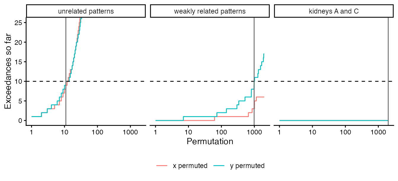

Running counts of exceedances against the permutation number for unrelated patterns, weakly related patterns and kidneys A and C, with the stopping line at 10 exceedances.

The dashed line is $h = 10$ , and the grey line marks where the adaptive run stopped (nPermutations of the adaptive result). The unrelated patterns reach 10 exceedances after 11 permutations and the weakly related pair after 984; kidneys A and C never exceed and run to the limit:

data.frame(example = names(adaptive),
           correlationCoef = sapply(adaptive, function(res) round(res$correlationCoef, 3)),
           nPermutations = sapply(adaptive, function(res) res$nPermutations),
           stop = sapply(adaptive, function(res) res$stop),
           pValuePermute = sapply(adaptive, function(res) signif(res$pValuePermute, 3)),
           row.names = NULL)
#>                   example correlationCoef nPermutations        stop
#> 1      unrelated patterns          -0.042            11 exceedances
#> 2 weakly related patterns           0.384           984 exceedances
#> 3         kidneys A and C           0.943          2000       limit
#>   pValuePermute
#> 1        0.9090
#> 2        0.0102
#> 3        0.0005

Because each permutation’s random numbers depend only on the seed, the gene and the permutation number, the adaptive run computed exactly the first $L$ permutations of the fixed run: it is the same experiment, stopped early.

Two directions, one p-value

Surrogates of x keep the autocorrelation of x but not of y, and the reverse for surrogates of y. STcompare runs both directions on the same permutation numbers, in lockstep, and stops a gene as soon as either direction reaches $h$ exceedances. The gene’s p-value, pValuePermute, is the larger of the two directions’ sequential p-values:

if one direction reached $h$ exceedances at permutation $L$ , pValuePermute is $h / L$ (the other direction, had it continued alone, could only have given a smaller value);
otherwise pValuePermute is $(\max(b_x, b_y) + 1) / (n + 1)$ .

The larger of two valid p-values is itself valid, whatever the dependence between them, so pValuePermute needs no assumption about how the two directions relate. Taking the larger value formalizes the rule of the original analyses, which called a gene significant when both directions were. pValuePermuteX and pValuePermuteY, $(b + 1) / (L + 1)$ for each direction at the common $L$ , are descriptive: they are not adjusted, and when a gene stops early, the direction that did not reach $h$ has an inflated value. (The legacy spatialCorrelationGeneExp() returns the same two raw columns for a fixed number of permutations, each adjusted across genes in pValuePermuteXAdj and pValuePermuteYAdj, and no combined p-value.)

Across the genes of a call, pValuePermuteAdj adjusts pValuePermute for multiple testing (Benjamini-Hochberg by default). With $G$ genes, the $k$ -th smallest p-value must be at most $\alpha k / G$ , so the smallest possible p-value, $1 / (n + 1)$ , matters when few genes are significant among many: see Parameters, performance and reproducibility.

Rarely detected genes

Step 5 exists because of genes detected in a handful of pixels. Without it, the surrogates are smoothed and mixed with Gaussian noise, so their values are close to normally distributed (surrogate = "gaussian", the surrogates of the legacy functions and of the published analyses). That suits a gene expressed over much of the tissue, but not a gene detected in a handful of pixels: the correlation of two such genes is decided by the few pixels where both are detected. Two unrelated genes that happen to share a detected pixel have a large correlation, and such coincidences happen far more often than the nearly normal values of gaussian surrogates produce extreme correlations. For example, two unrelated genes on the pixels of kidneys A and B, each detected in 3 pixels, one of which they share:

withValues <- function(values) {
  spe <- rast$A[, shared]
  assay(spe, "pixelval") <- matrix(values, nrow = 1,
                                   dimnames = list("Gene", shared))
  spe
}
sparseX <- sparseY <- numeric(length(shared))
sparseX[c(10, 100, 200)] <- c(3, 8, 5)
sparseY[c(100, 150, 250)] <- c(6, 2, 4)
sparse <- list(withValues(sparseX), withValues(sparseY))
gaussian <- compareSpatial(sparse, tests = "correlation", nPermutations = 999,
                           surrogate = "gaussian", minDetected = 0,
                           nThreads = 2, verbose = FALSE)
as.data.frame(gaussian)[, c("correlationCoef", "pValuePermute", "nPermutations")]
#>      correlationCoef pValuePermute nPermutations
#> Gene       0.6445649         0.001           999

None of the 999 gaussian surrogate pairs comes close to this correlation, so p is the smallest possible value. These genes have no spatial pattern, so shuffling the pixels of one of them gives the exact null distribution, and it shows how often such a coincidence happens by chance:

set.seed(2)
shuffled <- replicate(1e5, cor(sample(sparseX), sparseY))
exact <- mean(abs(shuffled) >= abs(gaussian$correlationCoef) * (1 - 1e-9))
exact
#> [1] 0.00333

(The tolerance counts the shuffles that give exactly the observed correlation, which cor() rounds differently for each arrangement of the values.) A correlation this large happens by chance about once in 300 shuffles, so the gaussian surrogates’ p-value, 0.001, is 3 times too small; with the default nPermutations = 10000 it would be 33 times too small. Remapped surrogates have the gene’s own values. For a gene without spatial structure the ranks of its surrogates are close to random, so its remapped surrogates are nearly plain shuffles of its values, and the test is close to the exact permutation test above, whatever the gene’s distribution. The defaults give a p-value of the right size:

remapped <- compareSpatial(sparse, tests = "correlation", nThreads = 2,
                           verbose = FALSE)
c(remapped = remapped$pValuePermute, exact = exact)
#>    remapped       exact 
#> 0.008216927 0.003330000

The remapped gene stopped after 1217 permutations with 10 exceedances, so its p-value is 10 / 1217, where the exact value predicts 4.1 exceedances. The remapped p-value errs on the safe side: the surrogate of a gene without spatial structure keeps a little smoothness, because the variogram matching takes the absolute value of a slope that is pure noise, so its null correlations are spread slightly more widely than those of plain shuffles. (Many rearrangements of a sparse gene give exactly the observed correlation; as in the exact test, such ties count as exceedances, within the rounding of cor().)

With gaussian surrogates, compareSpatial() does not test genes detected in fewer than $\sqrt{N}$ of the $N$ shared pixels of either sample (argument minDetected), here 17 of 273 pixels: the departure from the surrogates grows roughly as $N / (k_x k_y)$ for genes detected in $k_x$ and $k_y$ pixels, and the filter removes the genes for which it is largest, although genes detected in more pixels but still mostly zero can get p-values that are somewhat too small.

skipped <- compareSpatial(sparse, tests = "correlation", surrogate = "gaussian",
                          nThreads = 2, verbose = FALSE)
as.data.frame(skipped)[, c("pValuePermute", "status", "message")]
#>      pValuePermute  status
#> Gene            NA skipped
#>                                                                                                message
#> Gene detected in 3 (x) and 3 (y) of the 273 shared pixels; minDetected asks for 17 in each: not tested

With remapped surrogates, the default, no such filter is needed. In simulations on the pixels of the kidney and brain case studies, remapped surrogates kept $P(p \le \alpha) \le \alpha$ for independent genes detected in anywhere from 1% to 100% of the pixels, where gaussian surrogates were anti-conservative below about 10%, and they had the same power on correlated fields (bench/calibration-results.md in the source repository). minDetected therefore defaults to 0 with remapped surrogates: every gene that is not constant in a sample is tested, a gene without spatial structure costs about ten permutations, and the remapping itself, one sort of the $N$ values per surrogate, adds about 7% to the run time.

Spatial similarity

The correlation compares patterns and ignores the levels. The spatial similarity compares the levels at matched pixels. For each gene:

Threshold. The threshold of each sample is the gene’s minQuantile quantile (5% by default) over the shared pixels. A pixel is kept when its value is above the threshold in either sample: pixels where the gene is barely expressed in both samples would otherwise count as similar.
Log ratio. On the kept pixels, zeros are replaced by $10^{-4}$ and $l = \log_2(y / x)$ .
Classify. A pixel is similar if $|l| \le$ foldChange (1 by default, within two-fold), higher in x if $l <$ -foldChange, and higher in y if $l >$ foldChange.
Score. percentSimilarity is the share of similar pixels among the kept pixels, and percentDissimilarityX and percentDissimilarityY the shares of the other two classes (all three are proportions between 0 and 1, despite their names). If fewer than a share minPixels (10%) of the pixels are kept, the scores are NA.

These steps take a few lines of R for kidneys A and B, and give the value reported by compareSpatial():

keep <- x > quantile(x, 0.05) | y > quantile(y, 0.05)
x0 <- ifelse(x == 0, 1e-4, x)
y0 <- ifelse(y == 0, 1e-4, y)
l <- log2(y0[keep] / x0[keep])
c(byHand = mean(abs(l) <= 1), compareSpatial = ab$percentSimilarity)
#>         byHand compareSpatial 
#>      0.5347985      0.5347985

ggplot(data.frame(l = l), aes(l)) +
  annotate("rect", xmin = -1, xmax = 1, ymin = -Inf, ymax = Inf,
           fill = "steelblue", alpha = 0.2) +
  geom_histogram(bins = 40, fill = "grey40") +
  labs(x = "log2(B / A) of the kept pixels", y = "Pixels") +
  theme_classic()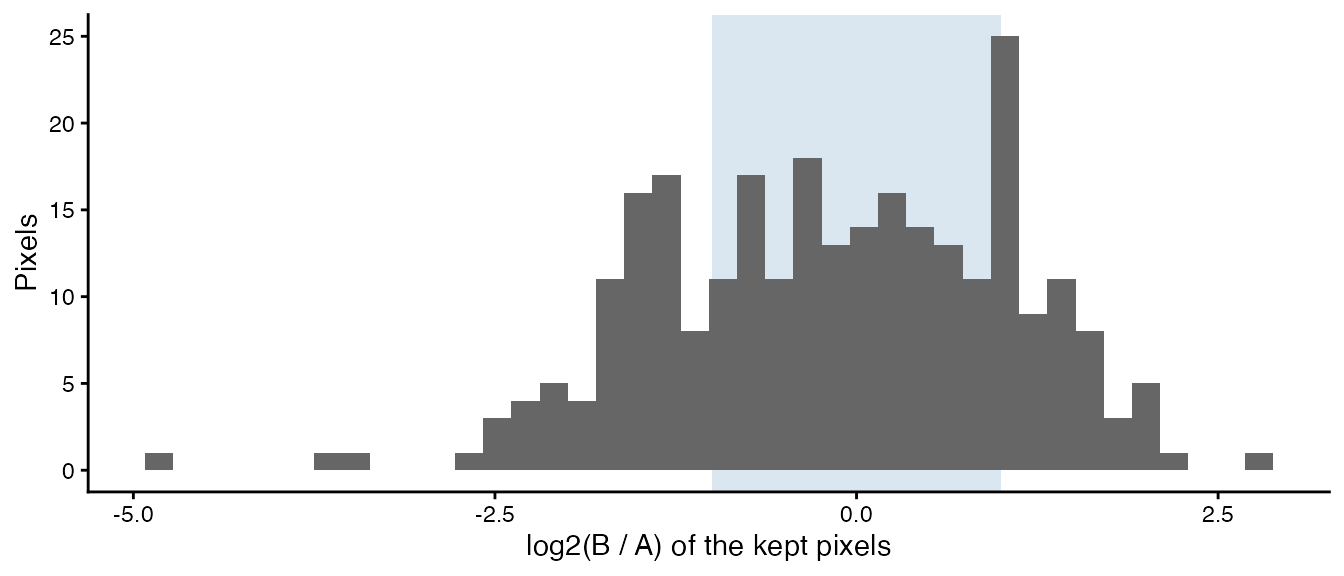

Histogram of the log2 ratios of B to A at the kept pixels; the shaded band between -1 and 1 holds the similar pixels.

The shaded band holds the similar pixels. The similarity is a description of the data and has no p-value. Because it compares levels, it needs values on a linear scale that are comparable between the samples (for example counts per million), not log-transformed values.

Summary

For each gene, compareSpatial():

takes the gene’s values on the pixels shared by the two samples, and skips the correlation test if the gene is constant in a sample (or, with gaussian surrogates, detected in too few pixels);
computes Pearson’s correlation, correlationCoef (and, for reference, the naive pValueNaive);
draws surrogates of each sample that keep its spatial autocorrelation (shuffle, smooth with each $\delta$ , match the variogram, keep delta star) and its values (remap), and correlates them with the other sample;
stops when either direction has exceedances null correlations at least as extreme as the observed correlation, or at nPermutations, and reports the larger of the two directions’ sequential p-values as pValuePermute (pValuePermuteX and pValuePermuteY hold $(b + 1) / (L + 1)$ for each direction);
adjusts pValuePermute across genes (pValuePermuteAdj);
computes the similarity of the levels at the kept pixels.

All genes share the expensive parts that depend only on the pixel coordinates (the smoothing operators and the variogram bins), and the permutations run on nThreads threads.

References

Clifton K, Jiang V, dos Santos Peixoto R, Singh S, Matsuura R, Rabb H, Fan J (2026). STcompare: comparative spatial transcriptomics data analysis of structurally matched tissues to characterize differentially spatially patterned genes. Bioinformatics 42(9):btag644. doi:10.1093/bioinformatics/btag644
Viladomat J, Mazumder R, McInturff A, McCauley DJ, Hastie T (2014). Assessing the significance of global and local correlations under spatial autocorrelation: a nonparametric approach. Biometrics 70(2):409-418. doi:10.1111/biom.12139
Theiler J, Eubank S, Longtin A, Galdrikian B, Farmer JD (1992). Testing for nonlinearity in time series: the method of surrogate data. Physica D 58(1-4):77-94. doi:10.1016/0167-2789(92)90102-S
Besag J, Clifford P (1991). Sequential Monte Carlo p-values. Biometrika 78(2):301-304. doi:10.1093/biomet/78.2.301
Benjamini Y, Hochberg Y (1995). Controlling the false discovery rate: a practical and powerful approach to multiple testing. Journal of the Royal Statistical Society B 57(1):289-300. doi:10.1111/j.2517-6161.1995.tb02031.x