Practical Machine Learning For Everyday Life
In this very practical R tutorial, we will see if we can use our machine learning skills to study something we enjoy in everyday life: wine.
We will use wine quality data from the UCI Machine Learning Repository. These two datasets are related to red and white variants of the Portuguese “Vinho Verde” wine. To start, read the data into R.
wine1.url <- "http://archive.ics.uci.edu/ml/machine-learning-databases/wine-quality/winequality-white.csv"
wine1 <- read.csv(wine1.url, header=TRUE, sep=';')
wine2.url <- "http://archive.ics.uci.edu/ml/machine-learning-databases/wine-quality/winequality-red.csv"
wine2 <- read.csv(wine2.url, header=TRUE, sep=';')
We will use only a subset of the data for demonstrative purposes. Each row is a different wine. Columns are features, including physicochemical measurements such as fixed acidity, volatile acidity, citric acid, residual sugar, chlorides, free sulfur dioxide, total sulfur dioxide, density, pH, sulphates, and alcohol, as well as a quality score between 0 and 10 and whether the wine is a red or white.
wine <- rbind(cbind(wine1[1:100,], type='white'), cbind(wine2[1:100,], type='red'))
wine$type <- as.factor(wine$type)
head(wine)
##   fixed.acidity volatile.acidity citric.acid residual.sugar chlorides
## 1           7.0             0.27        0.36           20.7     0.045
## 2           6.3             0.30        0.34            1.6     0.049
## 3           8.1             0.28        0.40            6.9     0.050
## 4           7.2             0.23        0.32            8.5     0.058
## 5           7.2             0.23        0.32            8.5     0.058
## 6           8.1             0.28        0.40            6.9     0.050
##   free.sulfur.dioxide total.sulfur.dioxide density   pH sulphates alcohol
## 1                  45                  170  1.0010 3.00      0.45     8.8
## 2                  14                  132  0.9940 3.30      0.49     9.5
## 3                  30                   97  0.9951 3.26      0.44    10.1
## 4                  47                  186  0.9956 3.19      0.40     9.9
## 5                  47                  186  0.9956 3.19      0.40     9.9
## 6                  30                   97  0.9951 3.26      0.44    10.1
##   quality  type
## 1       6 white
## 2       6 white
## 3       6 white
## 4       6 white
## 5       6 white
## 6       6 white
Binary classification
First, let’s see if we can train a binary classifier to differentiate between white and red wines. The caret package in R supports a huge number of models.
library(caret)
library(pROC)

head(names(getModelInfo()), n=30)
##  [1] "ada"            "AdaBag"         "AdaBoost.M1"    "adaboost"
##  [5] "amdai"          "ANFIS"          "avNNet"         "awnb"
##  [9] "awtan"          "bag"            "bagEarth"       "bagEarthGCV"
## [13] "bagFDA"         "bagFDAGCV"      "bam"            "bartMachine"
## [17] "bayesglm"       "bdk"            "binda"          "blackboost"
## [21] "blasso"         "blassoAveraged" "Boruta"         "bridge"
## [25] "brnn"           "BstLm"          "bstSm"          "bstTree"
## [29] "C5.0"           "C5.0Cost"
What ever model you choose, make sure it supports the type of modeling you want. We will use a gbm, which supports both classification and regression.
getModelInfo()$gbm$type
## [1] "Regression" "Classification"
First, we will try a binary classification problem. Can we train our gbm classifier to accurately distinguish red and white wines?
trait <- 'type'
features <- wine[, setdiff(colnames(wine), trait)]
head(features)
##   fixed.acidity volatile.acidity citric.acid residual.sugar chlorides
## 1           7.0             0.27        0.36           20.7     0.045
## 2           6.3             0.30        0.34            1.6     0.049
## 3           8.1             0.28        0.40            6.9     0.050
## 4           7.2             0.23        0.32            8.5     0.058
## 5           7.2             0.23        0.32            8.5     0.058
## 6           8.1             0.28        0.40            6.9     0.050
##   free.sulfur.dioxide total.sulfur.dioxide density   pH sulphates alcohol
## 1                  45                  170  1.0010 3.00      0.45     8.8
## 2                  14                  132  0.9940 3.30      0.49     9.5
## 3                  30                   97  0.9951 3.26      0.44    10.1
## 4                  47                  186  0.9956 3.19      0.40     9.9
## 5                  47                  186  0.9956 3.19      0.40     9.9
## 6                  30                   97  0.9951 3.26      0.44    10.1
##   quality
## 1       6
## 2       6
## 3       6
## 4       6
## 5       6
## 6       6
class <- wine[, trait]
head(class)
## [1] white white white white white white
## Levels: white red
ctrl <- trainControl(
  method="repeatedcv", ## 10 fold cross validation
  repeats=5, ## 5 repetitions of cross validation
  summaryFunction=twoClassSummary, ## two classes only
  classProbs=TRUE,
  savePred=TRUE
)

model <- train(
  x=features,
  y=class,
  method="gbm",
  trControl=ctrl,
  verbose=FALSE
)
Based on the ROC curve, it looks like we did pretty well!
plot.roc(model$pred$obs, model$pred$red)

## double check on new data
predict(model, newdata=wine1[100:110, 1:(ncol(wine1)-1)])
##  [1] white white white white white white white white white white white
## Levels: white red
predict(model, newdata=wine2[100:110, 1:(ncol(wine1)-1)])
##  [1] red red red red red red red red red red red
## Levels: white red
What features did our classifier find important and useful?
importance <- varImp(model, scale=FALSE)
print(importance)
## gbm variable importance
##
##                       Overall
## chlorides            81.02693
## volatile.acidity     20.41412
## total.sulfur.dioxide 15.50752
## density               9.51392
## sulphates             5.20135
## free.sulfur.dioxide   4.06884
## residual.sugar        2.94265
## pH                    1.73052
## fixed.acidity         0.25914
## citric.acid           0.15809
## alcohol               0.01027
## quality               0.00000
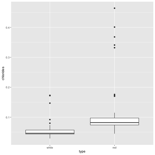
Our gbm classifier found that chlorides was very useful in distinguishing between red and white wines. Indeed, reds seem to have higher chloride levels than whites.
library(ggplot2)
ggplot(data=wine, aes(x=type, y=chlorides)) + geom_boxplot()
Regression
Now, let’s see if we can train a regression model to predict the wine’s quality given its various physicochemical measurements. We will use the red wine data only here since wine type is known to be a confounder for quality in this particular dataset.
trait <- 'quality'
features <- wine2[, setdiff(colnames(wine2), trait)]
head(features)
##   fixed.acidity volatile.acidity citric.acid residual.sugar chlorides
## 1           7.4             0.70        0.00            1.9     0.076
## 2           7.8             0.88        0.00            2.6     0.098
## 3           7.8             0.76        0.04            2.3     0.092
## 4          11.2             0.28        0.56            1.9     0.075
## 5           7.4             0.70        0.00            1.9     0.076
## 6           7.4             0.66        0.00            1.8     0.075
##   free.sulfur.dioxide total.sulfur.dioxide density   pH sulphates alcohol
## 1                  11                   34  0.9978 3.51      0.56     9.4
## 2                  25                   67  0.9968 3.20      0.68     9.8
## 3                  15                   54  0.9970 3.26      0.65     9.8
## 4                  17                   60  0.9980 3.16      0.58     9.8
## 5                  11                   34  0.9978 3.51      0.56     9.4
## 6                  13                   40  0.9978 3.51      0.56     9.4
class <- wine2[, trait]
head(class)
## [1] 5 5 5 6 5 5
ctrl <- trainControl(
  method="repeatedcv", ## 10 fold cross validation
  repeats=5, ## 5 repetitions of cross validation
  savePred=TRUE
)
model <- train(
  x=features,
  y=class,
  method="gbm",
  trControl=ctrl,
  verbose=FALSE
)
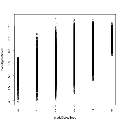
If we plot our predictions against the real quality score, we see a general positive correlation, but definitely less than perfect.
plot(model$pred$obs, model$pred$pred)
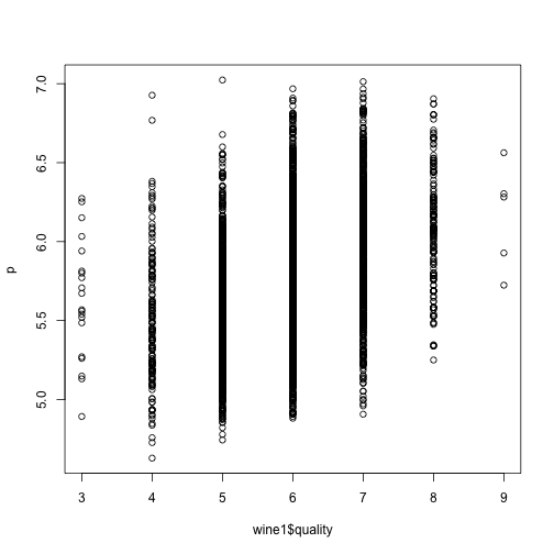
## double check by predicting on white wine data
p <- predict(model, newdata=wine1[, setdiff(colnames(wine2), trait)])
plot(wine1$quality, p)
What features did our model find important and useful?
importance <- varImp(model, scale=FALSE)
importance
## gbm variable importance
##
##                      Overall
## alcohol               727.07
## volatile.acidity      377.59
## sulphates             346.75
## total.sulfur.dioxide  198.10
## pH                    125.44
## chlorides             118.79
## citric.acid           113.84
## fixed.acidity          96.45
## density                91.38
## residual.sugar         86.11
## free.sulfur.dioxide    72.66
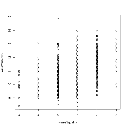
Alcohol?! Indeed, we see a general correlation between the quality of the wine and its alcohol content. Perhaps unsurprising haha ;)
plot(wine2$quality, wine2$alcohol)
Recent Posts
- AI-guided data visualization of gas prices in different geographical locations across the US over time on 04 May 2026
- The Mentorship Index on 01 March 2026
- Vibe coding with SEraster and STcompare to compare spatial transcriptomics technologies on 22 February 2026
- RNA velocity in situ infers gene expression dynamics using spatial transcriptomics data on 13 October 2025
- Analyzing ICE Arrest Data - Part 2 on 27 September 2025