Single Cell Clustering Comparison
So you aligned and quantified your single cell RNA-seq data. You QC-ed, normalized, and even batch corrected as needed. Now you want to identify transcriptional clusters. What clustering algorithm do you use?
Many specialized clustering methods for single cell RNA-seq data have been developed. Most come with sophisticated error modeling and other innovations. Still, they are generally grounded in some type of general k-means, graph-based, density-based, or hierarchical clustering.
So in this blog post, I will test out a few different general apporaches for identifying clusters in single cell RNA-seq data, namely: k-means, graph-based community detection, dbscan, and hierachical clustering. For demonstration, we will use the Patient B PBMC single cell RNA-seq data from 10X. PBMCs are nice because we have an expectation of what cell-types must be present and we know a number of markers for these cell-types (CD3E for T-cells, CD19 and CD20 for B-cells, etc). We can then compare the different clusters identified by various clustering approaches to what we know must be a cluster based on our knowledge of these cell markers.
Preparing the data
Let’s first quickly clean, normalize, and perform some dimensionality reduction on our PBMCs to get it into shape for clustering detection. We can then visualize a few of these known cell markers.
set.seed(0)

############# Sample data
library(MUDAN)
data(pbmcB)
## filter out poor genes and cells
cd <- cleanCounts(pbmcB,
                  min.reads = 10,
                  min.detected = 10,
                  verbose=FALSE)
## CPM normalization
mat <- normalizeCounts(cd,
                       verbose=FALSE)
## variance normalize, identify overdispersed genes
matnorm.info <- normalizeVariance(mat,
                                  details=TRUE,
                                  verbose=FALSE,
                                  alpha=0.2)
## log transform
matnorm <- log10(matnorm.info$mat+1)
## dimensionality reduction on overdispersed genes
pcs <- getPcs(matnorm[matnorm.info$ods,],
              nGenes=length(matnorm.info$ods),
              nPcs=30,
              verbose=FALSE)
## get tSNE embedding
emb <- Rtsne::Rtsne(pcs,
                    is_distance=FALSE,
                    perplexity=30,
                    num_threads=parallel::detectCores(),
                    verbose=FALSE)$Y
rownames(emb) <- rownames(pcs)
Based on our prior knowledge of marker genes, we can already tell that there must be distinct clusters corresponding to B-cells, T-cells subtypes, monocytes, and so forth. Indeed, we can see that CD20 (MS4A1) expression marks a distinct group of cells, presumably B-cells. And similarly, CD3E marks our T-cells, and so forth.
par(mfrow=c(3,3), mar=rep(2,4))
markers <- c('MS4A1', 'CD3E', 'IL7R', 'CCR7', 'CD8A', 'FCGR3A', 'CD14', 'HLA-DRA', "XCL1")
invisible(lapply(markers, function(g) {
  # plot binarized expression (on or off)
  plotEmbedding(emb, colors=(cd[g,]>0)*1,
              main=g, xlab=NA, ylab=NA,
              verbose=FALSE)
}))
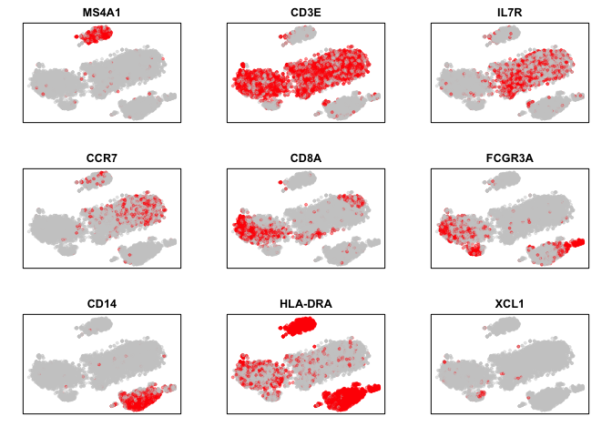
We can now try various cluster detection approaches and see if the identified clusters match what we expect based on marker expression.
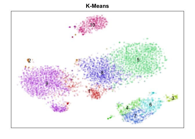
K-Means
First, we will use a simple k-means clustering
approach on our PCs.
With k-means clustering, a k must be provided a-priori to partition
your cells into k groups. Thus, the results rely heavily on your choice
of k. To be extra generous in our comparison, I tried a number of ks and
picked the best (as least visually) one to plot.
## k-means
set.seed(0)
com.km <- kmeans(pcs, centers=10)$cluster
par(mfrow=c(1,1), mar=rep(2,4))
plotEmbedding(emb, com.km,
              main='K-Means', xlab=NA, ylab=NA,
              mark.clusters=TRUE, alpha=0.1, mark.cluster.cex=1,
              verbose=FALSE)
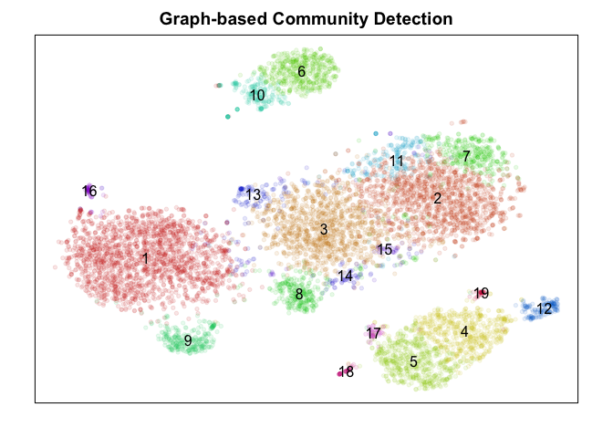
Graph-based community detection
Next, we will build a graph based on the nearest neighbor relationships in PC space. We can then apply graph-based community detection, specifically the Infomap method, to identify putative clusters. There are a number of other graph-based community detection algorithms you can use (Louvain, Walktrap, etc) but all will require building a graph. Here, I elected to build a graph from the 30 nearest neighbors in PC space for each cell.
## graph-based community detection
set.seed(0)
com.graph <- MUDAN::getComMembership(pcs,
                        k=30, method=igraph::cluster_infomap,
                        verbose=FALSE)
par(mfrow=c(1,1), mar=rep(2,4))
plotEmbedding(emb, com.graph,
              main='Graph-based Community Detection', xlab=NA, ylab=NA,
              mark.clusters=TRUE, alpha=0.1, mark.cluster.cex=1,
              verbose=FALSE)
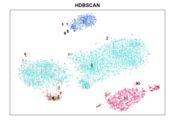
HDBSCAN
DBSCAN (or in this case, the hierarchical version) is nice in that it doesn’t require any expected number of clusters, such as k-mean’s k parameter, to be specified a priori. But I had a hard time getting sensible results using all PCs (too high dimensional) so I tried to reduce the dimensions considered to only PCS 1 to 5.
## Hierarchical DBSCAN
library(dbscan)
set.seed(0)
com.db <- hdbscan(pcs[,1:5], minPts=5)$cluster
names(com.db) <- rownames(pcs)
par(mfrow=c(1,1), mar=rep(2,4))
plotEmbedding(emb, com.db,
              main='HDBSCAN', xlab=NA, ylab=NA,
              mark.clusters=TRUE, alpha=0.1, mark.cluster.cex=1,
              verbose=FALSE)
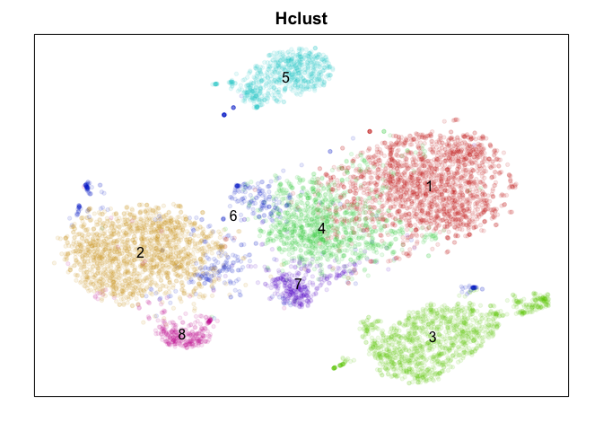
Hierarchical clustering
Hierarchical clustering or, alternatively biclustering (not shown) that clusters both cells and genes, builds tree relationship among cells that can then be cut at various heights to form clusters. Rather than choosing a cut height, I will use dynamic tree cutting. Of course, the choice of distance metric and agglomeration method for hierarchical clustering will still impact results. Here, I am using a 1 minus correlation in PC space to define the distance between cells and the Ward agglomeration method.
## Hierarchical clustering with dynamic tree cutting
library(dynamicTreeCut)
set.seed(0)
d <- as.dist(1-cor(t(pcs)))
hc <- hclust(d, method='ward.D')
com.hc <- cutreeDynamic(hc, distM=as.matrix(d), deepSplit=4, verbose=FALSE)
names(com.hc) <- rownames(pcs)
par(mfrow=c(1,1), mar=rep(2,4))
plotEmbedding(emb, com.hc,
              main='Hclust', xlab=NA, ylab=NA,
              mark.clusters=TRUE, alpha=0.1, mark.cluster.cex=1,
              verbose=FALSE)
In my own work, I am reaching the point where I must now consider not only the accuracy of a clustering algorithm but also its runtime and memory usage (primarily during software testing and development where I really value being able to iterate quickly). So we will also benchmark the runtime and memory usage of each cluster detection approach to get a sense of how well each method may scale as our datasets increase in size.
First, let’s benchmark runtime.
## try for different number of cells
ncells <- c(100, 200, 400, 800, 1600, 3200, 6400)

## k-means
rt.km <- sapply(ncells, function(vi) {
  start_time <- Sys.time()
  kmeans(pcs[1:vi,], centers=10)$cluster
  end_time <- Sys.time()
  return(end_time - start_time)
})

## graph-based community detection
rt.graph <- sapply(ncells, function(vi) {
  start_time <- Sys.time()
  getComMembership(pcs[1:vi,],
                   k=30, method=igraph::cluster_infomap,
                   verbose=FALSE)
  end_time <- Sys.time()
  return(end_time - start_time)
})

## HDBSCAN
rt.db <- sapply(ncells, function(vi) {
  start_time <- Sys.time()
  hdbscan(pcs[1:vi,1:5], minPts=10)$cluster
  end_time <- Sys.time()
  return(end_time - start_time)
})

## Hclust w/ dynamic tree cutting
library(dynamicTreeCut)
rt.hc <- sapply(ncells, function(vi) {
  start_time <- Sys.time()
  d <- as.dist(1-cor(t(pcs[1:vi,])))
  hc <- hclust(d, method='ward.D')
  com.hc <- cutreeDynamic(hc, distM=as.matrix(d), deepSplit=4, verbose=FALSE)
  names(com.hc) <- rownames(pcs)[1:vi]
  end_time <- Sys.time()
  return(end_time - start_time)
})
We will make an interactive plot here using
highcharter.
############# Highercharter
library(highcharter)
# Adapted from highcharter::export_hc() to not write to file
library(jsonlite)
library(stringr)
write_hc <- function(hc, name) {
  JS_to_json <- function(x) {
    class(x) <- "json"
    return(x)
  }
  hc$x$hc_opts <- rapply(object = hc$x$hc_opts, f = JS_to_json,
                         classes = "JS_EVAL", how = "replace")
  js <- toJSON(x = hc$x$hc_opts, pretty = TRUE, auto_unbox = TRUE,
               json_verbatim = TRUE, force = TRUE, null = "null", na = "null")
  js <- sprintf("$(function(){\n\t$('#%s').highcharts(\n%s\n);\n});",
                name, js)
  return(js)
}
# Helper function to write javascript in Rmd
# Thanks so http://livefreeordichotomize.com/2017/01/24/custom-javascript-visualizations-in-rmarkdown/
send_hc_to_js <- function(hc, hcid){
  cat(
    paste(
      '<span id=\"', hcid, '\"></span>',
      '<script>',
      write_hc(hc, hcid),
      '</script>',
      sep="")
  )
}

# Melt into appropriate format
df <- data.frame('graph'=rt.graph,
                 'km'=rt.km,
                 'db'=rt.db,
                 'hc'=rt.hc
                 )
dfm <- reshape2::melt(df)
dfm$ncell <- rep(ncells, 4)

# Plot
hcRT <- highchart() %>%
  hc_add_series(dfm, "line", hcaes(x = ncell, y = value, group = variable)) %>%
  hc_title(text = 'Runtime Comparison') %>%
  hc_legend(align = "right", layout = "vertical") %>%
  hc_xAxis(title = list(text = 'number of cells')) %>%
  hc_yAxis(title = list(text = 'runtime in seconds'))
send_hc_to_js(hcRT, 'hcRT')
K-means is quite fast! Graph-based community detection, which requires building a graph, is currently somewhat slow, though that may just be my poor implementation of the graph-construction approach from nearest neighbors. Similarly for hierarchical clustering, there may be faster C-based algorithms for calculating the distance matrices that could speed things up.
We can do the same for memory usage.
library(pryr)
## graph-based community detection
mem.graph <- sapply(ncells, function(vi) {
  return(mem_change(
  com <- getComMembership(pcs[1:vi,],
                   k=30, method=igraph::cluster_infomap,
                   verbose=FALSE)
  ))
})

## k-means
mem.km <- sapply(ncells, function(vi) {
  return(mem_change(
  com <- kmeans(pcs[1:vi,], centers=10)$cluster
  ))
})

## HDBSCAN
mem.db <- sapply(ncells, function(vi) {
  return(mem_change(
  com <- hdbscan(pcs[1:vi,1:5], minPts=5)$cluster
  ))
})

## Hclust w/ dynamic tree cutting
mem.hc <- sapply(ncells, function(vi) {
  return(
    mem_change(d <- as.dist(1-cor(t(pcs[1:vi,])))) +
    mem_change(hc <- hclust(d, method='ward.D')) +
    mem_change(com <- cutreeDynamic(hc, distM=as.matrix(d), deepSplit=4, verbose=FALSE))
  )
})
# Melt into appropriate format
df <- data.frame('graph'=mem.graph,
                 'km'=mem.km,
                 'db'=mem.db,
                 'hc'=mem.hc
                 )
dfm <- reshape2::melt(df)
dfm$ncell <- rep(ncells, 4)

# Plot
hcMem <- highchart() %>%
  hc_add_series(dfm, "line", hcaes(x = ncell, y = value, group = variable)) %>%
  hc_title(text = 'Memory Comparison') %>%
  hc_legend(align = "right", layout = "vertical") %>%
  hc_xAxis(title = list(text = 'number of cells')) %>%
  hc_yAxis(title = list(text = 'memory usage (log)'), type = "logarithmic")
send_hc_to_js(hcMem, 'hcMem')
Note that the y-axis is on the log scale! You definitely wouldn’t want to use hierachical clustering if you have millions of cells!
Conclusion
Judge for yourself! Which method did ‘better’? To really judge, we would want to check which method is better at identifying ‘stable’ clusters with truely differentially expressed genes. Only by looking for differentially expressed genes distinguishing each cluster would we be able to clarify which method properly split up the monocytes (marked by CD14) into putative subtypes. While k-means split monocytes into groups annotated 4, 6, and 7, graph-based community detection split into groups annotated as 4 and 5 which are not consistent with k-means, while the other methods did not identify any subtypes. DBSCAN appears to be better suited for identifying super small/rare populations such as groups marked 1, 8, and 9 as subtypes of B-cells (marked by CD20/MS4A1) but fails to distinguish between the large known T-cell subtypes (CD4, CD8 for example) at least using current settings. Hiearchical clustering is just too slow and memory intensive to be worthwhile in my opinion moving forward unless cells are downsampled or merged prior to clustering to reduce N.
What happens if we use different ks in our various cluster detection
approaches? Are some approaches more sensitive to parameter choices than
others? What if instead of PC space, we do our community detection in
the original expression space (using the entire normalized expression
matrix instead of PCs)? Try it out for yourself!
Recent Posts
- AI-guided data visualization of gas prices in different geographical locations across the US over time on 04 May 2026
- The Mentorship Index on 01 March 2026
- Vibe coding with SEraster and STcompare to compare spatial transcriptomics technologies on 22 February 2026
- RNA velocity in situ infers gene expression dynamics using spatial transcriptomics data on 13 October 2025
- Analyzing ICE Arrest Data - Part 2 on 27 September 2025