Using scVelo in R using Reticulate
Introduction
Although scRNA-seq has enabled us to characterize transcriptomes at
single cell resolution to identify transcriptionally distinct cell-types
and cell-states, it is a destructive protocol and thus only allows us to
capture a static snapshot in time. As we are often interested in how
cells change during dynamic processes such as differentiation, tumor
development, drug response, etc, we would like to infer some information
regarding directed temporal dynamics from this static snapshot. RNA
velocity analysis is a computational approach that allows us to
computationally predict where the cell is “heading” in terms of its gene
expression (e.g. predict the future transcriptional state of cells).
Details of RNA velocity analysis and modeling along with accompany
software as part of the velocyto.R R package can be found in the
original publication by La Manno et al.,
(2018). Recently, RNA
velocity analysis was expanded by Bergen et al
(2020) to further
enable inference of gene-specific rates of transcription, splicing and
degregation, accomodate transient cell-states, among other cool features
and has been made available as part of the scvelo Python package.
I am personally much more familiar with R programming and generally
prefer to stay within one programming language for reproducibility
purposes. So rather than switching to Python to use scvelo, in this
tutorial, I will demo the use scvelo from within R using R’s reticulate package.
Setting up
First, we will need to install reticulate. It also helps to have Conda
(https://docs.conda.io/en/latest/) installed to manage Python.
# install.packages("reticulate")
library(reticulate)
I previously created a Conda environment called r-velocity and
installed scvelo via:
# bash
pip install -U scvelo
You can double check in Python that the install worked using:
# bash
conda activate r-velocity
python
>>> import scvelo as scv
Now we can load up the appropriate Conda environment that has scvelo
installed.
conda_list()
##           name                                      python
## 1    anaconda3                   /opt/anaconda3/bin/python
## 2 r-reticulate /opt/anaconda3/envs/r-reticulate/bin/python
## 3   r-velocity   /opt/anaconda3/envs/r-velocity/bin/python
use_condaenv("r-velocity", required = TRUE)
scv <- import("scvelo")
scv$logging$print_version()
## Running scvelo 0.2.2 (python 3.8.5) on 2020-08-25 20:02.
scvelo
For demo purposes, we will work through the following tutorial (https://scvelo.readthedocs.io/) and work through how to interface with the results in R. We will download and use the built-in pancreas dataset.
adata <- scv$datasets$pancreas()
adata
## AnnData object with n_obs × n_vars = 3696 × 27998
##     obs: 'clusters_coarse', 'clusters', 'S_score', 'G2M_score'
##     var: 'highly_variable_genes'
##     uns: 'clusters_coarse_colors', 'clusters_colors', 'day_colors', 'neighbors', 'pca'
##     obsm: 'X_pca', 'X_umap'
##     layers: 'spliced', 'unspliced'
##     obsp: 'distances', 'connectivities'
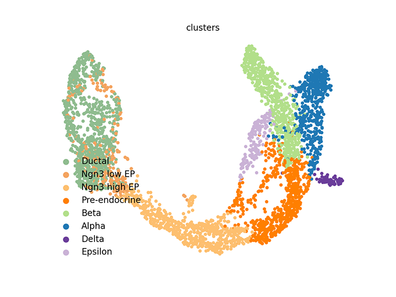
A UMAP embedding has already been generated and is accessible in the
pancreas dataset’s AnnData object. The same goes for cluster
annotations. We can plot results using scvelo’s plotting functions.
Note, this will result in a pop-up window.
scv$pl$scatter(adata, legend_loc='lower left', size=60)
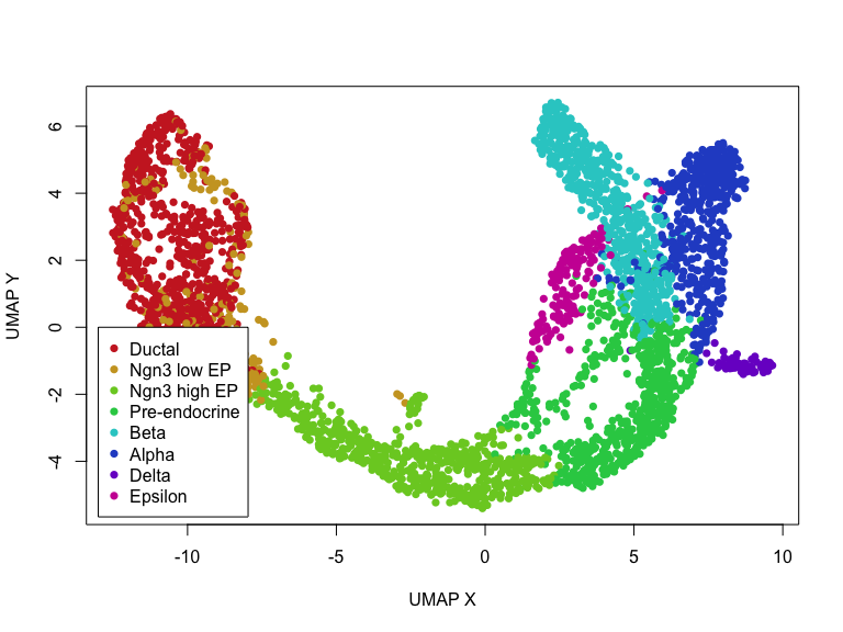
We can also access these elements and plot them within R.
## get embedding
emb <- adata$obsm['X_umap']
clusters <- adata$obs$clusters
rownames(emb) <- names(clusters) <- adata$obs_names$values

## get clusters, convert to colors
col <- rainbow(length(levels(clusters)), s=0.8, v=0.8)
cell.cols <- col[clusters]
names(cell.cols) <- names(clusters)

## simple plot
plot(emb, col=cell.cols, pch=16,
     xlab='UMAP X', ylab='UMAP Y')
legend(x=-13, y=0,
       legend=levels(clusters),
       col=col,
       pch=16)
Now, let’s actually run scvelo’s dynamic RNA velocity modeling on this
pancreas data from within R! Note, that the main difference in terms of
R function calls compared to python is now . are $. Other than that,
passing objects through py_to_r or r_to_py can fix a lot of errors.
## run scvelo dynamic model
scv$pp$filter_genes(adata) ## filter
scv$pp$moments(adata) ## normalize and compute moments
scv$tl$recover_dynamics(adata) ## model

## takes awhile, so uncomment to save
#adata$write('data/pancreas.h5ad', compression='gzip')
#adata = scv$read('data/pancreas.h5ad')
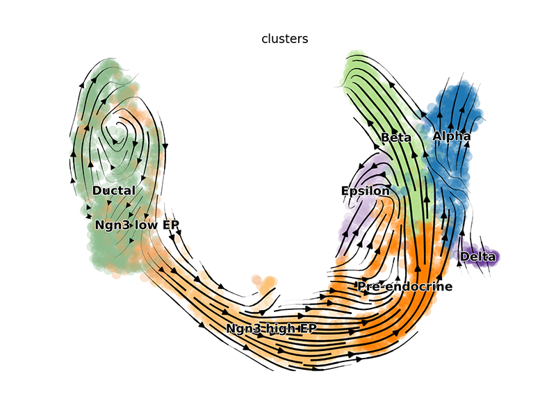
We can visualize the dynamic RNA velocities on the UMAP embedding using
scvelo’s plotting functions. Again, this will result in a pop-up
window.
## plot (creates pop up window)
scv$tl$velocity(adata, mode='dynamical')
scv$tl$velocity_graph(adata)
scv$pl$velocity_embedding_stream(adata, basis='umap')
## scv$pl$velocity_embedding_stream(adata, basis='pca') ## other embedding
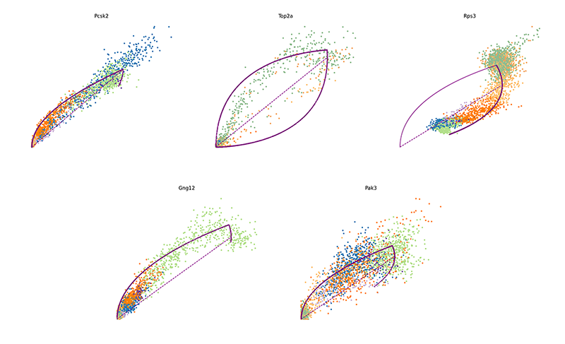
We can also pull out the top genes driving the dynamic RNA velocities.
## top dynamic genes
topgenes <- adata$var["fit_likelihood"]
topgenes_vals <- topgenes[,1]
names(topgenes_vals) <- rownames(topgenes)
topgenes_vals <- sort(topgenes_vals, decreasing=TRUE)
head(topgenes_vals)
##     Pcsk2     Top2a      Rps3     Gng12      Pak3       Ank
## 0.7811821 0.6639022 0.6355273 0.6131085 0.5956294 0.5955843
We can further visualize their phase diagrams using scvelo’s plotting
functions.
scv$pl$scatter(adata, basis=names(topgenes_vals)[1:5], ncols=5, frameon=FALSE)
velocyto.R
By working within R, we can also easily compare results with the
original, non-dynamic RNA velocity modeling with velocyto.R.
library(velocyto.R)
## Loading required package: Matrix
fit.quantile <- 0.1

## pull out spliced and unspliced matrices from AnnData
emat <- as.matrix(t(adata$layers['spliced']))
nmat <- as.matrix(t(adata$layers['unspliced']))
cells <- adata$obs_names$values
genes <- adata$var_names$values
colnames(emat) <- colnames(nmat) <- cells
rownames(emat) <- rownames(nmat) <- genes

## pull out PCA
pcs <- adata$obsm['X_pca']
rownames(pcs) <- cells
cell.dist <- as.dist(1-cor(t(pcs))) ## cell distance in PC space

## filter genes
gexp1 <- log10(rowSums(emat)+1)
gexp2 <- log10(rowSums(nmat)+1)
#plot(gexp1, gexp2)
good.genes <- genes[gexp1 > 2 & gexp2 > 1]
Now we can run the RNA velocity model using velocyto.R.
## velocyto model
rvel.cd <- gene.relative.velocity.estimates(emat[good.genes,], nmat[good.genes,],
                                            deltaT=1, kCells=30,
                                            cell.dist=cell.dist,
                                            fit.quantile=fit.quantile,
                                            mult=100)
## takes awhile, so uncomment to save
## save(rvel.cd, file="data/velocyto.RData")
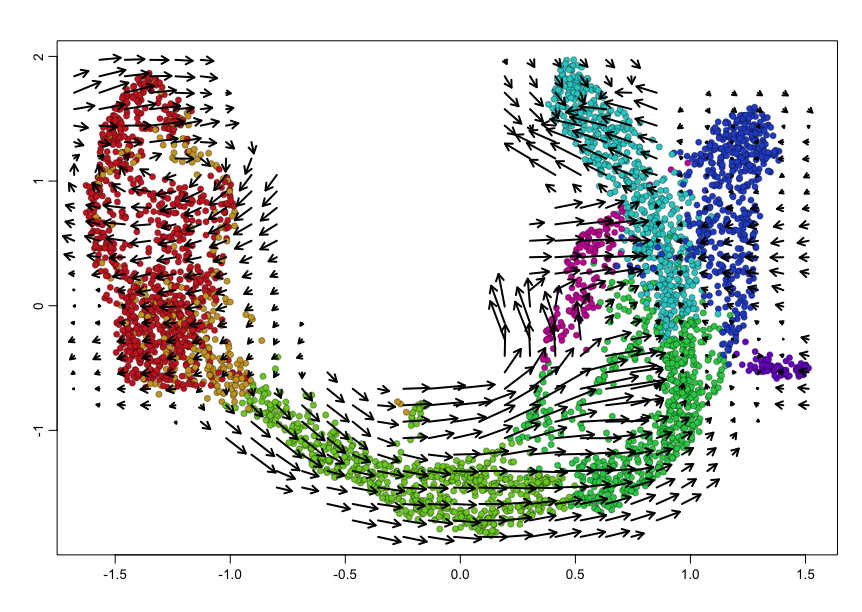
We can visualize the RNA velocities on the original UMAP embedding using
velocyto.R’s plotting functions.
## Plot on embedding
show.velocity.on.embedding.cor(scale(emb), rvel.cd,
                               n = 100,
                               scale='sqrt',
                               cex=1, arrow.scale=1, show.grid.flow=TRUE,
                               min.grid.cell.mass=0.5, grid.n=30, arrow.lwd=2,
                               cell.colors=cell.cols)
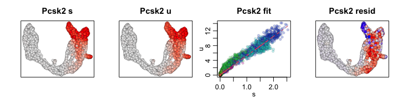
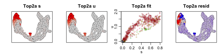
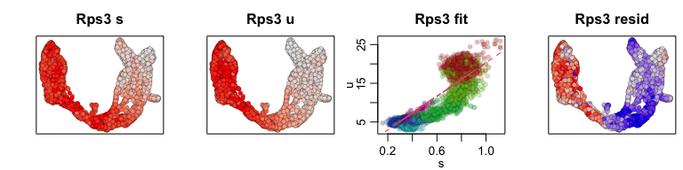
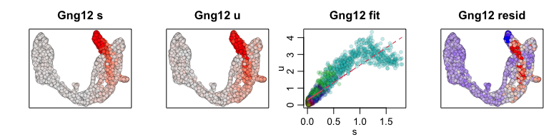
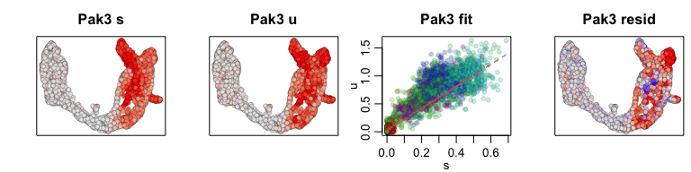
We can also visualize phase diagrams for the top dynamic genes from
scvelo using velocyto.R’s plotting functions.
## Gene plot
sapply(1:5, function(i) {
gene.relative.velocity.estimates(emat[good.genes,], nmat[good.genes,],
                                 kCells = 30,
                                 fit.quantile = fit.quantile,
                                 old.fit = rvel.cd,
                                 show.gene = names(topgenes_vals)[i],
                                 cell.emb = emb,
                                 cell.colors = cell.cols)
})
## calculating convolved matrices ... done
## calculating convolved matrices ... done
## calculating convolved matrices ... done
## calculating convolved matrices ... done
## calculating convolved matrices ... done
Additional tips
Alternatively, if we wanted to use our own data, we can create an
AnnData object such as follows. We can then use scvelo to run
analyses. If you are more comfortable in R like me, a lot of filtering,
clustering, and generating embeddings can be made within R and put into
the AnnData object such that scvelo is only used for the dynamic RNA
velocity component.
ad <- import("anndata", convert = FALSE)
dfobs <- data.frame(clusters, annotations)
rownames(dfobs) <- cells
dfvar <- data.frame(genes_attributes)
rownames(dfvar) <- genes
adata <- ad$AnnData(
  X=t(expression_matrix),
  obs=dfobs,
  var=dfvar,
  layers=list('spliced'=t(emat), 'unspliced'=t(nmat)),
  obsm=list('X_tsne'=emb, 'X_pca'=pcs$x[,1:2])
  )
Try it out for yourself!
Session info
sessionInfo()
## R version 4.0.2 (2020-06-22)
## Platform: x86_64-apple-darwin17.0 (64-bit)
## Running under: macOS Catalina 10.15.6
##
## Matrix products: default
## BLAS:   /Library/Frameworks/R.framework/Versions/4.0/Resources/lib/libRblas.dylib
## LAPACK: /Library/Frameworks/R.framework/Versions/4.0/Resources/lib/libRlapack.dylib
##
## locale:
## [1] en_US.UTF-8/en_US.UTF-8/en_US.UTF-8/C/en_US.UTF-8/en_US.UTF-8
##
## attached base packages:
## [1] stats     graphics  grDevices utils     datasets  methods   base
##
## other attached packages:
## [1] velocyto.R_0.6  Matrix_1.2-18   reticulate_1.16
##
## loaded via a namespace (and not attached):
##  [1] Rcpp_1.0.5          knitr_1.29          cluster_2.1.0
##  [4] magrittr_1.5        BiocGenerics_0.34.0 splines_4.0.2
##  [7] MASS_7.3-51.6       lattice_0.20-41     rlang_0.4.7
## [10] stringr_1.4.0       tools_4.0.2         parallel_4.0.2
## [13] grid_4.0.2          Biobase_2.48.0      nlme_3.1-148
## [16] mgcv_1.8-31         xfun_0.16           htmltools_0.5.0
## [19] yaml_2.2.1          digest_0.6.25       evaluate_0.14
## [22] rmarkdown_2.3       stringi_1.4.6       compiler_4.0.2
## [25] pcaMethods_1.80.0   jsonlite_1.7.0
Recent Posts
- AI-guided data visualization of gas prices in different geographical locations across the US over time on 04 May 2026
- The Mentorship Index on 01 March 2026
- Vibe coding with SEraster and STcompare to compare spatial transcriptomics technologies on 22 February 2026
- RNA velocity in situ infers gene expression dynamics using spatial transcriptomics data on 13 October 2025
- Analyzing ICE Arrest Data - Part 2 on 27 September 2025