The many ways to calculate Moran's I for identifying spatially variable genes in spatial transcriptomics data
In this blog post, I will compare 4 implementations of Moran’s I in R (MERINGUE, Rfast2, ape, and spdep) to identify spatially variable genes (SVGs) in spatial transcriptomics data.
## load packages
library(MERINGUE)
library(Rfast2)
library(ape)
library(spdep)
First, a little background
Recent technological advances have enabled high-throughput spatially resolved profiling of gene expression at single-cell and near single-cell resolution. This big data demands computational analysis to identify potentially interest biological signals. We previously developed MERINGUE, a computational framework and R package that uses spatial auto-correlation and cross-correlation statistics (including Moran’s I and modifications thereof) to identify genes with coordinated spatial variability in their gene expression patterns (ie. spatially variable genes or SVGs) among other screening tasks. Please refer to the manuscript for more details.
Moran’s I is a measure of spatial autocorrelation ie. a correlation in a signal’s intensity among nearby locations in space. In this cartoon, consider a grid of cells. For 5 example genes, high expression is visualized in black and low expression is denoted in white.
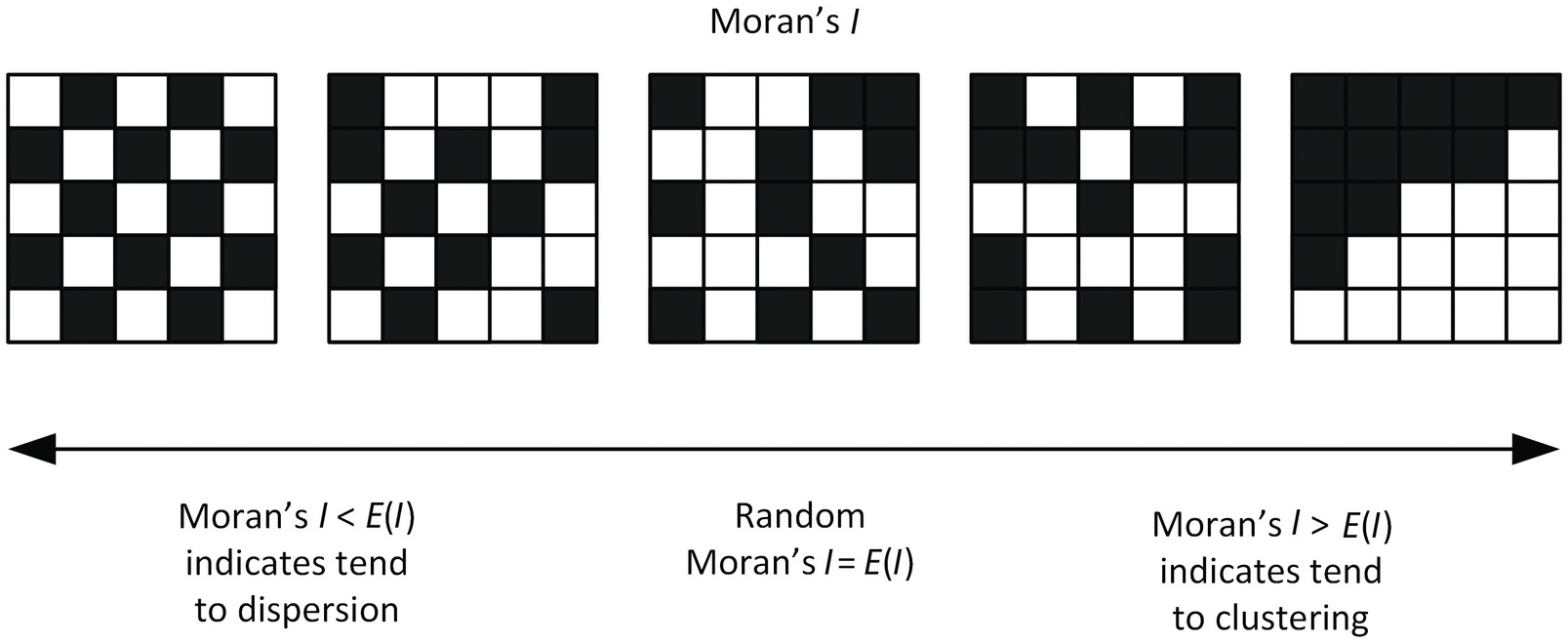
We may expect SVGs (genes with coordinated spatial variability in their gene expression patterns) to exhibit significantly higher than expected spatial autocorrelation that can be evaluated using Moran’s I.
However, as we note in our manuscript, even in context of spatial transcriptomics data analysis, there are actually many different ways to compute a Moran’s I statistic for a gene. In particular, how we define and mathematically encode whether two cells are close in space can influence results. We showed how using a binary spatial weight matrix derived from a Voronoi tesselation-based approach offers better performance compared to a distance-based spatial weight matrix for tissues where there is large variations in cell density that may confounder the spatial gene expression pattern. Again, please refer to the manuscript for more details.
However, recently, one of my students presented a bioRxiv preprint as part of our lab’s journal club that claimed Moran’s I performed poorly (only 19% accuracy!) for identifying SVGs based on simulated spatial transcriptomics data (where they simulated noise and true spatially patterned genes). Even in looking at their simulated data, I was surprised how Moran’s I could perform so poorly. Especially as we and many others have noted how Moran’s I performs well for identifying SVGs, the result was very suspicious to me. They did not use our MERINGUE implementation, but rather another tool that relied on implementations in Rfast2 and ape.
So I decided to spend some time comparing 4 different implementations of Moran’s I (MERINGUE, Rfast2, ape, and spdep) on some real spatial transcriptomics data to see if I could demonstrate a potential source of the discrepancy.
Getting our spatial transcriptomics data ready
For our exploration, let’s use a spatial transcriptomics mouse olfactory bulb dataset that’s built into the MERINGUE package.
data("mOB")
pos <- mOB$pos ## pixel positions
counts <- mOB$counts ## gene expression counts
head(pos)
##                        x      y
## GTTCCTGTGGTATTATGA  7.948 14.067
## GGTTTGTAAGTTAGCTCG 21.010 23.944
## ACCCGGCGTAACTAGATA 15.941 12.112
## ATATCGAAGTTTGGGTTT  8.957 11.091
## CCATAGTTAATGCGCTTC 16.945 11.075
## ATTAAGTAGCGCACGTTT 10.861 10.031
counts[1:5,1:5]
## 5 x 5 sparse Matrix of class "dgCMatrix"
##               GTTCCTGTGGTATTATGA GGTTTGTAAGTTAGCTCG ACCCGGCGTAACTAGATA
## 0610007N19Rik                  1                  .                  .
## 0610007P14Rik                  .                  1                  1
## 0610009B22Rik                  .                  .                  1
## 0610009D07Rik                  2                  1                  1
## 0610009L18Rik                  .                  .                  .
##               ATATCGAAGTTTGGGTTT CCATAGTTAATGCGCTTC
## 0610007N19Rik                  .                  .
## 0610007P14Rik                  .                  .
## 0610009B22Rik                  .                  1
## 0610009D07Rik                  3                  .
## 0610009L18Rik                  .                  .
Let’s make sure the cells in the counts matrix are in the same order as in the pos (for later, as other methods assume the spatial weight matrix w to be in the same order). We will also remove some genes that are not detected in a sufficient number of spots and spots that have too few genes for quality control purposes.
# make cells in same order
counts <- counts[, rownames(pos)]
# remove lowly expressed genes, bad spots
counts <- MERINGUE::cleanCounts(
	counts,
	min.detected = 5,
	min.lib.size = 100)
We will normalize our gene expression counts such that all spots have the same sequencing depth to prevent sequencing depth from confounding our SVG detection.
# in case we removed some cells
pos <- pos[colnames(counts),]
# CPM normalize
mat <- MERINGUE::normalizeCounts(counts, log=FALSE)
## Normalizing matrix with 260 cells and 13210 genes.
## normFactor not provided. Normalizing by library size.
## Using depthScale 1e+06
Next, we will construct a spatial weight matrix. For the sake of comparison, we will use the same Voronoi tesselation-based spatial weight matrix implemented in MERINGUE for all Moran’s I calculations across the 4 evaluated packages.
# Get neighbor-relationships
w <- getSpatialNeighbors(pos, filterDist = 2.5)
par(mfrow=c(1,1))
plotNetwork(pos, w)
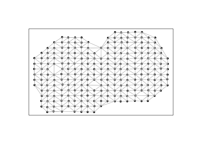
In this visualization, each point is a cell (technically a spot) for which we have measured gene expression, and cells are connected with a line if they are considered neighbors with a weight of 1 in the spatial weight matrix, and 0 otherwise.
Now we’re ready to run Moran’s I!
Calculating Moran’s I
Let’s first see how each package’s Moran’s I function can be used. For fun, I will also assess the time it takes to run each Moran’s I implementation.
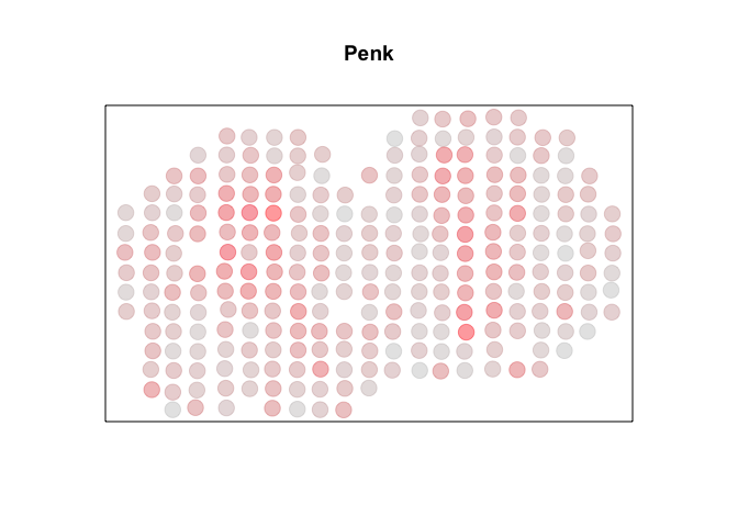
For demonstration purposes, we can cherry pick a known SVG, Penk. Visually, we can see a high degree of spatial autocorrelation, with cells that express Penk highly (in red) tending to be near other cells that also express Penk highly and cells that express Penk lowly (in grey) tending to be near other cells that also express Penk lowly. So we can check that each package’s Moran’s I is able to identify a significant autocorrelation.
g <- 'Penk'
x <- mat[g,]
par(mfrow=c(1,1))
MERINGUE::plotEmbedding(pos, col=x, main=g, cex=2)
Moran’s I in MERINGUE
In the Moran’s I implementation in MERINGUE, given a gene’s expression x and the spatial weight matrix w, I used C++ via Rcpp to calculate for the observed I statistic as well as the expected and standard deviation of the I statistic under no spatial autocorrelation. I can then use a Z-test assuming asymptotic normality to compare the observed I statistic to the expected and standard deviation of the I statistic under a null hypothesis to derive a p-value.
Note, in MERINGUE, the alternative hypothesis is a one-sided greater Z-test by default. This means, we are rejecting the null when the observed I statistic is larger than what is expected under the null hypothesis; that is gene x exhibits more spatial autocorrelation than what is expected at random. Altenrative two.sided and one-sided less test are also availble, though I will show later why these alternative hypotheses may be less appropriate in identifying SVGs.
## C++ implementation of Moran's I in MERINGUE package
start_time <- Sys.time()
I <- MERINGUE::moranTest(x, w)
end_time <- Sys.time()
print(end_time - start_time)
## Time difference of 0.001333952 secs
print(I)
##     observed     expected           sd      p.value
##  0.368746559 -0.003861004  0.036736603  0.000000000
It takes us a fraction of a second and output the observed I statistic as well as the expected and standard deviation of the I statistic under no spatial autocorrelation along with an associated p-value.
Alternatively, instead of solving for the expected and standard deviation of the I statistic under no spatial autocorrelation, we can use a permutation test and derive a permutation p-value. In this case, I am permuting the gene expression x a total of N=1e3 times, calculating an I statistic for each permutation, and comparing the observed to the permuted I statistics to derive a permutation p-value. Again, note we are doing a one-sided greater permutation test, which means we are evaluating if our observed I statistics is greater than what we expect by chance based on permutations.
## Native R implementation permutation-based Moran's I in MERINGUE package
start_time <- Sys.time()
Ip <- MERINGUE::moranPermutationTest(x, w, N=1e3)
end_time <- Sys.time()
print(end_time - start_time)
## Time difference of 0.5554221 secs
print(Ip)
##      observed      expected            sd       p.value             N
##  3.687466e-01 -8.640044e-04  3.830120e-02  9.990010e-04  1.000000e+03
Note, this is implemented using native R and therefore quite slow…so we can stop using it for the remainder of the comparisons.
Moran’s I in Rfast2
In the Moran’s I implementation in Rfast2, given a gene’s expression x and the spatial weight matrix w, a permutation-approach across R permutations is used to derive a p-value.
## Rfast2's permutation-based Moran's I
start_time <- Sys.time()
## note no way to specify one-sided test
I2 <- Rfast2::moranI(x, w, R = 1e3)
end_time <- Sys.time()
print(end_time - start_time)
## Time difference of 0.00155592 secs
print(I2)
##           Moran's I permutation p-value
##        0.3687465593        0.0009756098
Notably, Rfast2 also uses permutation test but it uses C++ to speed up functions to it is much faster than the native R implementation we saw previously!
However, the Rfast2 implementaiton of Moran’s I does not give an option to do a one-sided ‘greater’ permutation test. The only option is to perform a two-sided test. Again, I will show later this may be problematic for identifying SVGs.
Moran’s I in ape
In the Moran’s I implementation in ape, given a gene’s expression x and the spatial weight matrix w, the observed I statistic as well as the expected and standard deviation of the I statistic under no spatial autocorrelation is computed and a Z-test is used to derive a p-value. Note, in ape, the alternative hypothesis is a two.sided test by default. I will specify a one-sided ‘greater’ test here so we can focus on evaluating whether this gene exhibits more spatial autocorrelation than what is expected. The results are returned as a list object so I use unlist to convert to a vector.
## ape's Moran's I
start_time <- Sys.time()
I3 <- unlist(ape::Moran.I(x, w, alternative='greater'))
end_time <- Sys.time()
print(end_time - start_time)
## Time difference of 0.003234863 secs
print(I3)
##     observed     expected           sd      p.value
##  0.368746559 -0.003861004  0.036736603  0.000000000
Moran’s I in spdep
In the Moran’s I implementation in spdep is quite similar ape, though it requires the spatial weights to be provided as a listw object. So we will convert our w matrix using the mat2listw function. Note, in spdep, the alternative hypothesis is a one-sided greater test by default. The results are returned as an htest object so I will just pull out the slots I need and reorganize into a data frame.
start_time <- Sys.time()
I4.info <- spdep::moran.test(x, mat2listw(w, style="W"))
I4 <- c(I4.info$estimate, p.value = I4.info$p.value)
end_time <- Sys.time()
print(end_time - start_time)
print(I4)
## Time difference of 0.01602888 secs
print(I4)
## Moran I statistic       Expectation          Variance           p.value
##      3.687466e-01     -3.861004e-03      1.349578e-03      1.785843e-24
Promisingly, all implementations of Moran’s I give the same observed I statistic. The p-values also all consistently suggest that this gene significant, as expected.
Now, let’s apply to all genes!
Evaluating the full transcriptome
This runtime difference becomes much more evident as we assess all genes in our dataset.
Moran’s I in MERINGUE
In MERINGUE, I implemented a function getSpatialPatterns that uses C++ via Rcpp to loop through all the genes, run Moran’s I, and concatenate the results into an Rcpp arma::mat that is then cast into an R-native dataframe. I also calculate an adjusted p-value p.adj to take into consideration multiple testing correction.
start_time <- Sys.time()
## Looping in done in C++
I <- MERINGUE::getSpatialPatterns(mat, w, verbose = FALSE)
end_time <- Sys.time()
print(end_time - start_time)
## Time difference of 7.651681 secs
head(I)
##                  observed     expected         sd     p.value      p.adj
## 0610007N19Rik  0.002143838 -0.003861004 0.03623405 0.434187182 0.80771233
## 0610007P14Rik  0.049436633 -0.003861004 0.03674413 0.073458547 0.34868394
## 0610009B22Rik  0.016352591 -0.003861004 0.03653620 0.290046645 0.69153992
## 0610009D07Rik -0.022507855 -0.003861004 0.03680182 0.693811345 0.92206899
## 0610009L18Rik  0.080426641 -0.003861004 0.03489022 0.007850426 0.07874269
## 0610009O20Rik -0.016099332 -0.003861004 0.03676587 0.630384559 0.91138650
It takes us less than 10 seconds to evaluate all the genes in our dataset!
Alternatively, we could also perform the looping in native R, calling our C++ implementation of Moran’s I from previously, and concatenate the results into a dataframe.
start_time <- Sys.time()
## Alternatively, run Moran's I in C++ but do looping in R
Il <- do.call(rbind, lapply(rownames(mat), function(i){
  MERINGUE::moranTest(mat[i,], w)
}))
rownames(Il) <- rownames(mat)
end_time <- Sys.time()
print(end_time - start_time)
## Time difference of 36.58219 secs
head(Il)
##                  observed     expected         sd     p.value
## 0610007N19Rik  0.002143838 -0.003861004 0.03623405 0.434187182
## 0610007P14Rik  0.049436633 -0.003861004 0.03674413 0.073458547
## 0610009B22Rik  0.016352591 -0.003861004 0.03653620 0.290046645
## 0610009D07Rik -0.022507855 -0.003861004 0.03680182 0.693811345
## 0610009L18Rik  0.080426641 -0.003861004 0.03489022 0.007850426
## 0610009O20Rik -0.016099332 -0.003861004 0.03676587 0.630384559
Note the calculated numbers are all the same but it took us over 3x longer to do so!
Moran’s I in Rfast2
Anyways, now let’s try Rfast2, which also uses C++ to speed up functions.
start_time <- Sys.time()
I2 <- do.call(rbind, lapply(rownames(mat), function(i){
  Rfast2::moranI(mat[i,], w, R = 1e3)
}))
rownames(I2) <- rownames(mat)
I2 <- data.frame(I2)
end_time <- Sys.time()
print(end_time - start_time)
## Time difference of 40.31104 secs
head(I2)
##                  Moran.s.I permutation.p.value
## 0610007N19Rik  0.002143838          0.94146341
## 0610007P14Rik  0.049436633          0.08682927
## 0610009B22Rik  0.016352591          0.53951220
## 0610009D07Rik -0.022507855          0.41170732
## 0610009L18Rik  0.080426641          0.01658537
## 0610009O20Rik -0.016099332          0.54634146
The Rfast implementation is indeed quite fast for permutation testing but still 3x slower than the MERINGUE C++ implementation.
Moran’s I in ape
Now, let’s try ape, which again implements Moran’s I in native R.
start_time <- Sys.time()
I3 <- do.call(rbind, lapply(rownames(mat), function(i){
  unlist(ape::Moran.I(mat[i,], w, alternative='greater'))
}))
rownames(I3) <- rownames(mat)
I3 <- data.frame(I3)
end_time <- Sys.time()
print(end_time - start_time)
## Time difference of 1.090592 mins
head(I3)
##                  observed     expected         sd     p.value
## 0610007N19Rik  0.002143838 -0.003861004 0.03623405 0.434187182
## 0610007P14Rik  0.049436633 -0.003861004 0.03674413 0.073458547
## 0610009B22Rik  0.016352591 -0.003861004 0.03653620 0.290046645
## 0610009D07Rik -0.022507855 -0.003861004 0.03680182 0.693811345
## 0610009L18Rik  0.080426641 -0.003861004 0.03489022 0.007850426
## 0610009O20Rik -0.016099332 -0.003861004 0.03676587 0.630384559
Moran’s I in spdep
And finally, let’s try spdep, which also implements Moran’s I in native R.
start_time <- Sys.time()
I4 <- do.call(rbind, lapply(rownames(mat), function(i){
  I4.info <- spdep::moran.test(mat[i,], mat2listw(w, style="W"))
  c(I4.info$estimate, p.value = I4.info$p.value)
}))
rownames(I4) <- rownames(mat)
I4 <- data.frame(I4)
end_time <- Sys.time()
print(end_time - start_time)
## Time difference of 3.457737 mins
I probably should’ve removed the mat2listw call to outside the loop to avoid recreating a listw object every single time. Let’s try that again.
start_time <- Sys.time()
listw <- mat2listw(w, style="W")
I4 <- do.call(rbind, lapply(rownames(mat), function(i){
  I4.info <- spdep::moran.test(mat[i,], listw)
  c(I4.info$estimate, p.value = I4.info$p.value)
}))
rownames(I4) <- rownames(mat)
I4 <- data.frame(I4)
end_time <- Sys.time()
print(end_time - start_time)
## Time difference of 1.524801 mins
head(I4)
##               Moran.I.statistic  Expectation    Variance     p.value
## 0610007N19Rik       0.002143838 -0.003861004 0.001312906 0.434187182
## 0610007P14Rik       0.049436633 -0.003861004 0.001350131 0.073458547
## 0610009B22Rik       0.016352591 -0.003861004 0.001334894 0.290046645
## 0610009D07Rik      -0.022507855 -0.003861004 0.001354374 0.693811345
## 0610009L18Rik       0.080426641 -0.003861004 0.001217327 0.007850426
## 0610009O20Rik      -0.016099332 -0.003861004 0.001351729 0.630384559
Much better. Expectedly, these native R implementations are quite slow (in my impatient opinion), taking over a minute.
Personally, I think the conclusion is clear:

Identifying SVGs from these implementations of Moran’s I
As noted previously, we can identify SVGs as genes with significant Moran’s Is (p-value so low that we can reject the null hypothesis of no spatially patterning). However, based on the printed head outputs, you may have already noticed some discrepancies between the p-values from Rfast2 and the other implementations. As we are all calculating the same statistic, using the same w neighbor-weight matrix, we should get all the same results…right? Recall, we are performing a one-sided greater test in MERINGUE, ape, and spdep, but Rfast2 only allows us to do a two-sided test. Let’s see what difference this makes.
Instead of looking at the first few genes, let’s assess the correspondence between at all of them using data visualization.
## compare
par(mfrow=c(2,3))
plot(I$observed, I2$Moran.s.I,
     xlab = 'MERINGUE', ylab = 'Rfast2',
     main = 'Moran\'s I statistic') ## i statistic correspondence
plot(I$observed, I3$observed,
     xlab = 'MERINGUE', ylab = 'ape',
     main = 'Moran\'s I statistic') ## i statistic correspondence
plot(I2$Moran.s.I, I3$observed,
     xlab = 'Rfast2', ylab = 'ape',
     main = 'Moran\'s I statistic') ## i statistic correspondence

## p value correspondence between MERINGUE and ape
plot(-log10(I$p.value), -log10(I3$p.value),
     xlab = 'MERINGUE', ylab = 'ape',
     main = '-log10(p-value)')
## p value correspondence between MERINGUE and Rfast2
plot(-log10(I$p.value), -log10(I2$permutation.p.value),
     xlab = 'MERINGUE', ylab = 'Rfast2',
     main = '-log10(p-value)')
## p value correspondence between Rfast2 and ape
plot(-log10(I2$permutation.p.value), -log10(I3$p.value),
     xlab = 'Rfast2', ylab = 'ape',
     main = '-log10(p-value)')
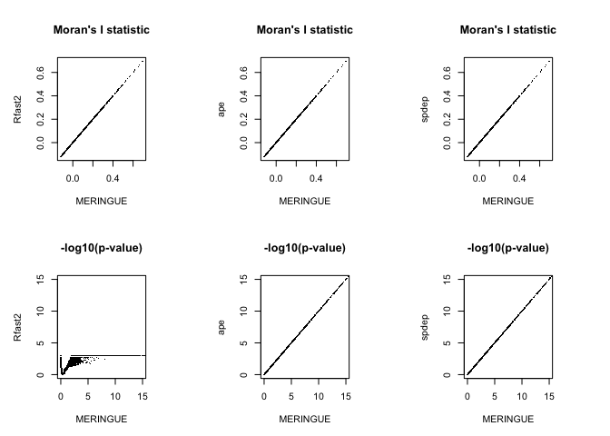
Note that the Moran’s I statistics exactly the same across all evaluated implementations. Great!
However, while the p-values for MERINGUE, ape, and spdep agree, the p-values from Rfast2 differ quite a bit…different. And not just because it plateaus at 3 because this is a permutation p-value and I only used 1e3 permutations. The lack of agreement is because of that one-sided vs two-sided test difference.
Erroneous SVGs?
Let’s take a closer look at the disagreement. Specifically, let’s look at some genes for which the Moran’s I p-value from Rfast2 suggests significance (and thus an SVG) but MERINGUE (and ape and spdep since their p-values are the same) does not suggest significance (and thus not an SVG).
## Rfast2 results
test <- which(I2$permutation.p.value < 0.05)
## MERINGUE results
foo <- I[test,]
head(foo[order(foo$p.value, decreasing=TRUE),])
##          observed     expected         sd   p.value     p.adj
## Akt1s1 -0.1198926 -0.003861004 0.03685240 0.9991796 0.9991796
## Tomm5  -0.1147985 -0.003861004 0.03675918 0.9987276 0.9988032
## Meaf6  -0.1102675 -0.003861004 0.03662001 0.9981678 0.9983189
## Usp42  -0.1049741 -0.003861004 0.03593356 0.9975527 0.9977793
## Doc2a  -0.1054168 -0.003861004 0.03651763 0.9972905 0.9975926
## Vps35  -0.1040892 -0.003861004 0.03679018 0.9967783 0.9971557
Let’s visualize one gene Akt1s1.
par(mfrow=c(1,1))
g <- "Akt1s1"
MERINGUE:::plotEmbedding(pos, col=mat[g,], cex=2, main=g)
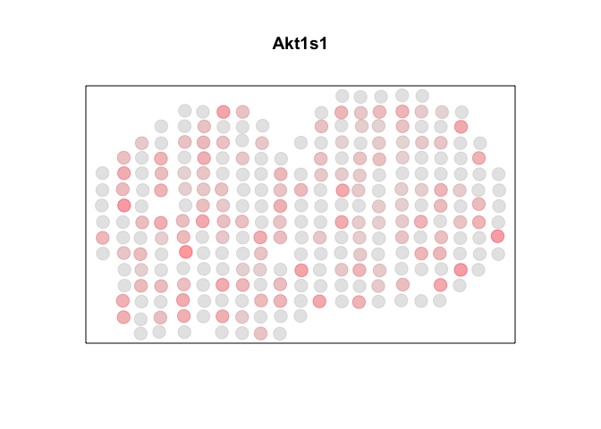
Indeed, Rfast2 identified this gene as significant (p-value < 0.05) whereas MERINGUE, ape, and spdep did not.
## Rfast2 says significant
print(I2[g,])
##         Moran.s.I permutation.p.value
## Akt1s1 -0.1198926        0.0009756098
## MERINGUE says not significant
print(I[g,])
##          observed     expected        sd   p.value     p.adj
## Akt1s1 -0.1198926 -0.003861004 0.0368524 0.9991796 0.9991796
## ape says not significant
print(I3[g,])
##          observed     expected        sd   p.value
## Akt1s1 -0.1198926 -0.003861004 0.0368524 0.9991796
## spdep says not significant
print(I4[g,])
##        Moran.I.statistic  Expectation  Variance   p.value
## Akt1s1        -0.1198926 -0.003861004 0.0013581 0.9991796
This gene doesn’t look very spatially autocorrelated to me. Indeed, it is actually spatially…anti-autocorrelated (ie. perfectly dispersed)! That means, cells (or in this case spots) that are spatially close together tend to have differing expression magnitudes of this gene. I’m not actually quite sure how to interpret the biological meaning this pattern, but I wouldn’t consider it an SVG.
We can also confirm that this difference is just from using a one-sided or two-sided test, by running the implementation of Moran’s I in ape using a two.sided test as well (which is the default).
unlist(ape::Moran.I(mat[g,], w)) ## alternative='two.sided' default
##     observed     expected           sd      p.value
## -0.119892581 -0.003861004  0.036852402  0.001640835
Now we get a significant p-value from this two-sided test. We can also confirm that this significance is due to a significant dispersion by using a one-sided less test. So the observed I statistic is indeed significantly less than what we expect under the null model, suggesting spatial dispersion.
unlist(ape::Moran.I(mat[g,], w, alternative='less')) ## one sided less
##      observed      expected            sd       p.value
## -0.1198925812 -0.0038610039  0.0368524023  0.0008204174
Conclusions/speculations
So it is possible that the preprint in question simply ran a two.sided instead of a one-sided greater test and therefore identified a large number of significantly spatially dispersed genes (that were likely in the “noise” group) as SVGs, resulting in the poor performance.
It is also worth noting that the Rfast2, ape, and spdep implementations of Moran’s I do not have built-in checks for whether x and w have cells in the same order. In the event x and w do not have cells in the same order, results from Rfast2, ape, and spdep would also be incorrect. We can demonstrate this by shuffling the order of x. Note that now Rfast2, ape, and spdep no longer identify Penk as significant because of my induced user error.
g <- 'Penk'
set.seed(0)
x <- sample(mat[g,]) ## shuffle order
MERINGUE::moranTest(x, w) ## has internal checks based on cell names
##    observed     expected           sd      p.value
## 0.368746559 -0.003861004  0.036736603  0.000000000
Rfast2::moranI(x, w, R = 1e3)
##          Moran's I permutation p-value
##         0.04091384          0.10048780
unlist(ape::Moran.I(x, w, alternative='greater'))
##    observed     expected           sd      p.value
## 0.040913838 -0.003861004  0.036736603  0.111458662
spdep::moran.test(x, mat2listw(w, style="W"))
## Moran I test under randomisation

## data:  x
## weights: mat2listw(w, style = "W")

## Moran I statistic standard deviate = 1.2188, p-value = 0.1115
## alternative hypothesis: greater
## sample estimates:
## Moran I statistic       Expectation          Variance
##       0.040913838      -0.003861004       0.001349578
Lastly, it may also be that the preprint used a different spatial encoding for w that impacted the performance (without the original code, it is hard to say for certain…)
Based on this exploration, I hope it’s clear that just because a paper says they’re using Moran’s I to detect SVGs, they can actually mean many different things! A well described methods section (or ideally code) should help clarify the exact w and sided-test they used.
Additional fun tidbits
- I implemented
MERINGUE’s C++ version of Moran’s I by studyingape’s native R implementation code. If you want an example of well written code that actually reads like the original mathematical formulation, I highly recommend readingape::Moran.I, as it emphasizes clarity/readability over concision/one-liners. - I also implemented
MERINGUE’s C++ version of Moran’s I because I thoughtapewas too slow. If someone can make an even faster implementation, perhaps in Rust, please feel free to reach out and let me know! - I compared runtime but not memory efficiency across all 4 implementations. It is worth noting,
MERINGUE,Rfast2, andapeuse an NxN spatial weight matrix where N is the number of cells (or spots) in your spatial transcriptomics data. As spatially resolved transcriptomics technologies continue to improve, enabling the profiling of more and more cells, this has presented a major memory issue. I suspectspdep’slistwmay actually be more memory efficient here. In my lab, we are currently shifting towards rasterization preprocessing as a way of aggregating data prior to Moran’s I, which we recently showed was an effective time and memory-saving approach. But perhaps a sparse spatial weight matrix implementation would also be beneficial in the long run.
Try it out for yourself!
Recent Posts
- The Mentorship Index on 01 March 2026
- Vibe coding with SEraster and STcompare to compare spatial transcriptomics technologies on 22 February 2026
- RNA velocity in situ infers gene expression dynamics using spatial transcriptomics data on 13 October 2025
- Analyzing ICE Arrest Data - Part 2 on 27 September 2025
- Analyzing ICE Detention Data from 2021 to 2025 on 10 July 2025