Analyzing ICE Detention Data from 2021 to 2025
The ability to code and explore big datasets are generally useful skills that transfer well beyond our work of biomedical spatial omics analysis. In this blog post, I analyze publicly available datasets from the U.S. Immigration and Customs Enforcement (ICE) Enforcement and Removal Operations (ERO) website. I learned about these datasets from KPBS San Diego’s border reporter Gustavo Solis. The dataset comprises Excel spreadsheets that summarize information about who is currently being held in immigration detention and where. Let’s download these spreadsheets and take a look for ourselves in R and make some plots to help us visualize the data.
Getting started: download and read in data
I downloaded the data from the bottom of the page at https://www.ice.gov/detain/detention-management. There is a lot of sheets in each Excel file so I will focus on the ‘Facilities’ sheet as Gustavo recommends. Unfortunately the spreadsheets are not perfectly standardized. Some times the ‘Facilities’ sheet is the 4th sheet, some times the 7th. The sheets can have different names “Facilities EOY24” or “Facilities FY22”. Some times there are headers in the first 5 lines, some times first 6. So they must be read in and inspected manually rather than in some more automated loop. I focus on the datasets from 2021 onward to avoid the COVID-19 pandemic-associated effects of 2020. It is also worth keeping in mind that the 2025 data is only til June 20th and therefore does not represent an entire year.
library(readxl)
fy21 = readxl::read_xlsx('FY21-detentionstats.xlsx', sheet=4, skip=6)
fy22 = readxl::read_xlsx('FY22-detentionstats.xlsx', sheet=7, skip=6)
fy23 = readxl::read_xlsx('FY23_detentionStats.xlsx', sheet=8, skip=5)
fy24 = readxl::read_xlsx('FY24_detentionStats.xlsx', sheet=8, skip=6)
fy25 = readxl::read_xlsx('FY25_detentionStats06202025.xlsx', sheet=7, skip=6)
head(fy25)
## # A tibble: 6 × 28
##   Name           Address City  State   Zip AOR   `Type Detailed` `Male/Female` `FY25 ALOS` `Level A` `Level B` `Level C`
##   <chr>          <chr>   <chr> <chr> <dbl> <chr> <chr>           <chr>               <dbl>     <dbl>     <dbl>     <dbl>
## 1 ADAMS COUNTY … 20 HOB… NATC… MS    39120 NOL   DIGSA           Female/Male         49.8      1890.     258.      12.7
## 2 ADELANTO ICE … 10250 … ADEL… CA    92301 LOS   CDF             Female/Male         37.9      16.5      11.9      52.9
## 3 ALAMANCE COUN… 109 SO… GRAH… NC    27253 ATL   IGSA            Female/Male         2.55      6.02      3.24      5.77
## 4 ALEXANDRIA ST… 96 GEO… ALEX… LA    71303 NOL   STAGING         Male                2.61      143.      50.3      75.7
## 5 ALLEGANY COUN… 4884 S… BELM… NY    14813 BUF   IGSA            Female/Male         11.1      3.46      0.151     0.0438
## 6 ALLEN PARISH … 7340 H… OBER… LA    70655 NOL   IGSA            Male                63.5      98.5      29.8      32.0
## # ℹ 16 more variables: `Level D` <dbl>, `Male Crim` <dbl>, `Male Non-Crim` <dbl>, `Female Crim` <dbl>,
## #   `Female Non-Crim` <dbl>, `ICE Threat Level 1` <dbl>, `ICE Threat Level 2` <dbl>, `ICE Threat Level 3` <dbl>,
## #   `No ICE Threat Level` <dbl>, Mandatory <dbl>, `Guaranteed Minimum` <chr>, `Last Inspection Type` <chr>,
## #   `Last Inspection End Date` <chr>, `Pending FY25 Inspection` <chr>, `Last Inspection Standard` <chr>,
## #   `Last Final Rating` <chr>
Note each row is an ICE detention facility. We generally have the name
and location information of each facility along with summary
quantifications, such as the number of men who have criminal records
(Male Crim), men without criminal records (Male Non-Crim), and so
forth. Additional information about what the column names and acronym
entries mean can be found on the ice.gov website.
Let’s put all these datasets together and see what are some shared features that we can compare across years.
fylist <- list(fy21, fy22, fy23, fy24, fy25)
names(fylist) <- 2021:2025

# intersect all columns
Reduce(intersect, lapply(fylist, colnames))
##  [1] "Name"                 "Address"              "City"                 "State"                "Zip"
##  [6] "AOR"                  "Type Detailed"        "Male/Female"          "Level A"              "Level B"
## [11] "Level C"              "Level D"              "Male Crim"            "Male Non-Crim"        "Female Crim"
## [16] "Female Non-Crim"      "ICE Threat Level 1"   "ICE Threat Level 2"   "ICE Threat Level 3"   "No ICE Threat Level"
## [21] "Mandatory"            "Guaranteed Minimum"   "Last Inspection Type"
Who is being detained?
Let’s focus first on quantifying the total number of men who have criminal records, men without criminal records, women who have criminal records, and women without criminal records who have been detained across all ICE facilities every year. To do this, we will loop through our spreadsheets and sum up the categories of interest.
# columns of interest
categories = c("Male Crim", "Male Non-Crim", "Female Crim", "Female Non-Crim")
# loop through spreadsheets
df <- do.call(rbind, lapply(categories, function(category) {
  sapply(fylist, function(fytest) {
    sum(fytest[,category], na.rm=TRUE)
  })
}))
rownames(df) <- categories
# look at our results
print(df)
##                     2021       2022       2023       2024       2025
## Male Crim       5444.147  4693.3286  7536.4274  9355.6995 11897.4064
## Male Non-Crim   9619.400 13374.8640 16534.2247 22209.4098 26029.2749
## Female Crim      317.450   225.9547   398.1918   543.9727   808.1753
## Female Non-Crim 2911.208  3050.1643  3679.3260  4168.3333  4790.9681
We now have a count of the number of people detained per year for each category. Let’s make a plot to visualize these trends over time.
library(ggplot2)
library(reshape2)

dfreshape <- reshape2::melt(df)
gg1 <- ggplot(dfreshape, aes(y=value, x=Var2, col=Var1)) +
  facet_grid(cols=vars(Var1)) +
  geom_line() +
  labs(title = paste0('Number of ICE detainees by Category Over Time'),
       x = 'year',
       y = 'number of people') +
  theme_bw(base_size = 13) +
  theme(legend.position='none') +
  theme(axis.text.x = element_text(angle = 90, vjust = 0.5, hjust=1))

print(gg1)
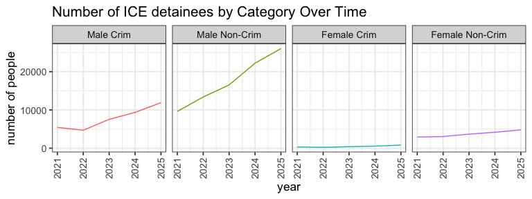
This data visualization makes salient in terms of who is being detained in these ICE facilities that:
- there are many more men who are detained in these ICE facilities compared to women
- there are many more men without criminal records who are detained in these ICE facilities compared to men with criminal records
How do trends break down geographically by ICE facilities?
We may be interested in how these trends break down in terms of specific ICE facilities and where they may be located geographically. There are well over 100 ICE facilities. It will be left as an exercise to the student to create a trend plot like the one above but for each facility rather than all ICE facilities aggregated together. But for now, I will focus on making one summary visualization.
Specifically, I want to make a summary visualization that makes salient whether there are any geographic patterns with respect to the rate of detention for non-criminal versus criminal detainees. I will focus on men who are detained since they make up the bulk of detainees. Since the spreadsheets include information about the facility’s zipcode, I will use this to visualize each facility as a point on a map. I will then quantify the ratio or fold-change of non-criminals versus criminals and encode this log2 fold-change as each point’s color. I also want to keep track of the size of each facility as each point’s radius.
The first step is to create a dataframe that has all the information I want, including each facility’s zipcode, location in terms of longtitude and latitude, ratio of non-criminal versus criminal detainees, size in terms of total detainees, as well as name and year for book-keeping.
library(zipcodeR)
library(dplyr)
library(tidyr)

alldata <- do.call(rbind, lapply(2021:2025, function(year) {
  fytest <- fylist[[as.character(year)]]

  # get facility names
  facs <- na.omit(unique(fytest$Name))

  # calculate ratio of criminal to non-criminal
  facratio <- sapply(facs, function(fac) {
    (sum(fytest[fytest$Name == fac, "Male Non-Crim"], na.rm=TRUE)+1)/
      (sum(fytest[fytest$Name == fac, "Male Crim"], na.rm=TRUE)+1)
  })
  names(facratio) <- facs
  # take a log2 (fold change)
  facratio <- log2(facratio)

  # where are these facilities based on zip code
  zip <- as.character(fytest$Zip)
  names(zip) <- fytest$Name

  # keep track of size as total detainees
  size <- rowSums(fytest[, c("Male Non-Crim", "Male Crim", "Female Non-Crim", "Female Crim")])
  names(size) <- fytest$Name

  # make into data frame
  zipdata <- data.frame(
    name = names(facratio),
    zip = zip[names(facratio)],
    size = size[names(facratio)],
    ratio = facratio
  )

  # use zipcodeR to get lat/lon
  zipcoords <- reverse_zipcode(zipdata$zip) %>%
    select(zipcode, lat, lng) %>%
    rename(zip = zipcode)
  zipdata <- left_join(zipdata, zipcoords, by = "zip") %>% drop_na()
  zipdata <- zipdata[order(zipdata$ratio),]

  # keep track of year and return
  zipdata$year = year
  return(zipdata)

}))
head(alldata)
##                                    name   zip      size     ratio   lat     lng year
## 55 CLINTON COUNTY CORRECTIONAL FACILITY 17745  75.57222 -5.666491 41.30  -77.40 2021
## 49                   GOLDEN STATE ANNEX 93250  98.44722 -4.787219 35.70 -119.20 2021
## 75     MESA VERDE ICE PROCESSING CENTER 93301  35.83889 -3.584733 35.39 -119.02 2021
## 91                     YUBA COUNTY JAIL 95901  13.41667 -3.499015 39.20 -121.50 2021
## 31       ADELANTO ICE PROCESSING CENTER 92301 228.88611 -3.071722 34.60 -117.50 2021
## 90    HONOLULU FEDERAL DETENTION CENTER 96819  13.85556 -3.050941 21.35 -157.88 2021
Given this organized data, we can visualize the results on a map of the United States, using facetting to make a different plot per year but keeping the same legend so we can more readily visually compare across plots to appreciated trends.
library(ggplot2)
library(scales)
library(maps)

# get map to visualize on US map
us_map <- map_data("state")

# plot using ggplot
gg <- ggplot() +
  geom_polygon(data = us_map, aes(x = long, y = lat, group = group),
               fill = "gray95", color = "white") +
  geom_point(data = alldata, aes(x = lng, y = lat, size=size, col=ratio, group=name), alpha = 0.7) +
  scale_color_gradient2(low = 'blue', mid = 'grey', high='red', limits=c(-2,2), oob=squish) +
  scale_size_binned() +
  coord_quickmap(xlim = c(-125, -66), ylim = c(25, 50)) +
  theme_void(base_size = 13) +
  theme(plot.title = element_text(hjust = 0.5),
        strip.text = element_text(size = 15),
        legend.position="bottom",
        legend.box = "vertical",
        legend.key.width = unit(2, "cm"),
        plot.margin = margin(1,1,1.5,2.5, "cm")) +
  labs(title = "ICE Detention Facilities Across the USA",
       x = "Longitude", y = "Latitude",
       color = "Log2(Male Non-Crim / Male Crim) Detainees",
       size = "Number of Total Detainees") +
  facet_grid(row=vars(year))

print(gg)
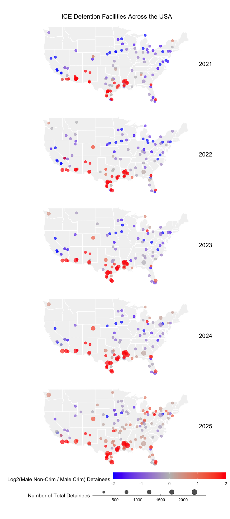
Are there any interesting spatial trends you can glean from this data visualization? For example, there appears to be be more non-criminal compared to criminal detainees in ICE facilities along the border (points are more red than blue). Over time, though particularly in 2025, there appears to be an increase in the number, size, and ratio of non-criminal compared to criminal detainees (new points appear, blue points become more red and get bigger over time) in ICE facilities farther from the border such as in Kentucky, Missouri, Iowa, Ohio, and Pennsylvania.
What types of facilities have the largest ratio of non-criminal to criminal detainees?
Let’s focus further on the ICE facilities with more than 4x more non-criminal than criminal detainees.
# focus on 2025, ratio of non-criminal to criminal (log2 > 2) ie. more than 4x more non-criminal than criminal
topfac <- alldata[alldata$year == '2025' & alldata$ratio >= 2,]
head(topfac)
##                                      name   zip      size    ratio    lat      lng year
## 1052           OTAY MESA DETENTION CENTER 92154 1345.8008 2.377976 32.600 -117.000 2025
## 126    SAN LUIS REGIONAL DETENTION CENTER 85349  145.2112 2.383933 32.492 -114.784 2025
## 139                 TORRANCE/ESTANCIA, NM 87016  435.9841 2.472860 34.700 -106.100 2025
## 234     CIBOLA COUNTY CORRECTIONAL CENTER 87021  227.5737 2.567710 35.171 -107.892 2025
## 674  IMPERIAL REGIONAL DETENTION FACILITY 92231  665.6295 2.589767 32.700 -115.500 2025
## 934          MONROE COUNTY DETENTION-DORM 48161  100.0956 2.612757 41.900  -83.500 2025
There are many ‘types’ of ICE facilities. Each ICE facility has an associated ‘Type - Detailed’.
For example:
- CDF = Contract Detention Facility: a facility that is owned by a private company and contracted directly with the government.
- USMS CDF = Private facility contracted with the US Marshal Service.
- USMS IGA = Intergovernment agreement in which ICE agrees to utilize an already established US Marshal Service contract.
- IGSA = Inter-governmental Service Agreement: a facility operated by state/local government(s) or private contractors and falls under public ownership.
- DIGSA = Dedicated IGSA.
- JUVENILE = Juvenile: an IGSA facility capable of housing juveniles (separate from adults) for a temporary period of time.
- FAMILY = Family: a facility in which families are able to remain together while awaiting their proceedings.
- SPC = Service Processing Center: a facility that is owned by the government and staffed by a combination of federal and contract employees.
type <- as.factor(fy25$`Type Detailed`)
names(type) <- fy25$Name
head(type)
##            ADAMS COUNTY DET CENTER     ADELANTO ICE PROCESSING CENTER ALAMANCE COUNTY DETENTION FACILITY
##                              DIGSA                                CDF                               IGSA
##        ALEXANDRIA STAGING FACILITY               ALLEGANY COUNTY JAIL ALLEN PARISH PUBLIC SAFETY COMPLEX
##                            STAGING                               IGSA                               IGSA
## Levels: BOP CDF DIGSA DOD IGSA MOC SPC STAGING USMS CDF USMS IGA
Let’s count the number of each type of ICE facility for the facilities with 4x more non-criminal than criminal detainees. We can compare to the total number of each type of ICE facility to see if the ones with 4x more non-criminal than criminal detainees are over-represented or enriched in any participate type.
topfactype <- sort(table(type[topfac$name])/table(type), decreasing=TRUE)
print(topfactype)
##   USMS CDF      DIGSA        CDF        SPC       IGSA   USMS IGA        BOP        DOD        MOC    STAGING
## 0.50000000 0.28000000 0.21428571 0.20000000 0.14285714 0.02857143 0.00000000 0.00000000 0.00000000 0.00000000
It seems that ICE facilities with 4x more non-criminal than criminal detainees are most likely to be of the “USMS CDF” type and also of the “CDF” type. These are private facilities owned and operated by private companies.
Which private companies are profiting from the detention of non-criminal people?
Let’s look into the specific ICE facilities that have these high ratios non-criminal to criminal detainees and are of the “USMS CDF” or “CDF” type.
specfac <- topfac$name[type[topfac$name] %in% c('USMS CDF', 'CDF')]
print(specfac)
## [1] "OTAY MESA DETENTION CENTER"
## [2] "IMPERIAL REGIONAL DETENTION FACILITY"
## [3] "HOUSTON CONTRACT DETENTION FACILITY"
## [4] "RIO GRANDE DETENTION CENTER"
If we Google the names of these ICE facilities, we can find that:
- OTAY MESA DETENTION CENTER and HOUSTON CONTRACT DETENTION FACILITY are owned and operated by CoreCivic, a private prison company that is publicly-traded on the stock exchange under CXW
- RIO GRANDE DETENTION CENTER is owned and operated by GEO Group, a private prison company that is publicly-traded on the stock exchange under GEO
- IMPERIAL REGIONAL DETENTION FACILITY is owned by Imperial Valley Gateway Center, LLC and operated by Management and Training Corporation (MTC), both of which are private companies but not publicly-traded
We can then cross-reference the stock prices for CoreCivic’s CXW and Geo Group’s GEO from the past year since these are publicly traded companies:
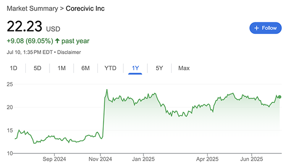
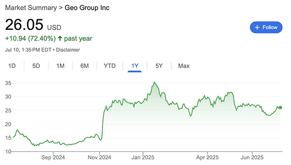
Presidential elections were held in the United States on November 5, 2024.
Thoughts and conclusions
We have performed an exploratory data analysis of publicly available ICE datasets. As with any exploratory data analysis, be they for biomedical data or ICE detention data, the results allow us to form a working hypothesis that we can then iterate on with additional data collection and analyses. It will be left up as an exercise to the student to form these hypotheses for themselves.
Try it out for yourself!
Try and take a look at the data for yourself. See what additional hypotheses you may be able to generate from exploring these datasets.
Some questions to explore include:
- Criminal records can mean many things from petty theft to murder. Therefore, ICE provides summaries of detainees by ‘threat level’, ranging from 1 (most severe) to 3 (least severe). Are there any trends in the threat levels of criminal detainees over time? Or geographically?
- The spreadsheets contain additional columns like ‘Guaranteed Minimum’ and ‘Mandatory.’ What do these mean and are there any trends over time? Or geographically?
- The spreadsheets contain additional columns like ‘Level A’, ‘Level B’, etc. What do these mean and are there any trends over time? Or geographically?
- Explore a different sheet other than the one associated with ICE facilities.
- Integrate additional census data to determine how the number of non-criminal detainees is associated with the immigrant population size.
Recent Posts
- The Mentorship Index on 01 March 2026
- Vibe coding with SEraster and STcompare to compare spatial transcriptomics technologies on 22 February 2026
- RNA velocity in situ infers gene expression dynamics using spatial transcriptomics data on 13 October 2025
- Analyzing ICE Arrest Data - Part 2 on 27 September 2025
- Analyzing ICE Detention Data from 2021 to 2025 on 10 July 2025