Analyzing ICE Arrest Data - Part 2
In this blog post, I continue to demonstrate how to analyze publicly available datasets related to U.S. Immigration and Customs Enforcement (ICE). This time, I take advantage of publicly available data from deportationdata.org from The Deportation Data Project, which collects and posts public, anonymized U.S. government immigration enforcement datasets obtained from the Freedom of Information Act. Importantly, this dataset contains individual-level information rather than group summaries.
Getting started: download and read in data
We will use readxl to read in the excel spreadsheet of the Arrests
data from Sep. 2023 to Late
Jul. 2025.
library(readxl)
arrests <- read_excel('~/Downloads/arrests-latest.xlsx', sheet=1)
head(arrests)
## # A tibble: 6 × 23
##   apprehension_date   apprehension_state apprehension_aor          final_program
##   <dttm>              <chr>              <chr>                     <chr>
## 1 2023-09-01 00:00:00 CALIFORNIA         San Francisco Area of Re… ERO Criminal…
## 2 2023-09-01 00:00:00 SOUTH CAROLINA     Atlanta Area of Responsi… ERO Criminal…
## 3 2023-09-01 00:00:00 <NA>               <NA>                      Alternatives…
## 4 2023-09-01 00:00:00 <NA>               <NA>                      Alternatives…
## 5 2023-09-01 00:00:00 <NA>               Phoenix Area of Responsi… Detained Doc…
## 6 2023-09-01 00:00:00 <NA>               <NA>                      Non-Detained…
## # ℹ 19 more variables: final_program_group <chr>, apprehension_method <chr>,
## #   apprehension_criminality <chr>, case_status <chr>, case_category <chr>,
## #   departed_date <dttm>, departure_country <chr>, final_order_yes_no <chr>,
## #   final_order_date <dttm>, birth_year <dbl>, citizenship_country <chr>,
## #   gender <chr>, apprehension_site_landmark <chr>, unique_identifier <chr>,
## #   apprehension_date_time <dttm>, duplicate_likely <lgl>, file_original <chr>,
## #   sheet_original <chr>, row_original <dbl>
Note each row is an individual that has been arrested by ICE. We have
information regarding their apprehension date (apprehension_date),
apprehension method (apprehension_method), criminality on a level of 1
to 3 as defined by ICE (apprehension_criminality), among other
information.
Let’s use data visualizations to address some questions and make certain
trends in this data more salient. We will use tidyverse and dplyr to
help us keep the code tidy. I will create a new data frame with only the
information I want - the apprehension date (date), apprehension
criminality (criminality), and appehension method (method) just to
keep the output more legible.
Note that this dataset only contains information for a part of July, so the entire month is not well represented compared to previous months. Therefore, I will also filter for data from only the full months.
library(tidyverse)
library(dplyr)

arrests_df <- data.frame(
  date = arrests$apprehension_date,
  criminality = arrests$apprehension_criminality,
  method = arrests$apprehension_method)

arrests_df <- arrests_df %>%
  filter(date < as.Date("2025-07-01")) # filter to full months

head(arrests_df)
##         date                  criminality                    method
## 1 2023-09-01         1 Convicted Criminal CAP Federal Incarceration
## 2 2023-09-01   2 Pending Criminal Charges   CAP Local Incarceration
## 3 2023-09-01 3 Other Immigration Violator    ERO Reprocessed Arrest
## 4 2023-09-01 3 Other Immigration Violator    ERO Reprocessed Arrest
## 5 2023-09-01 3 Other Immigration Violator    ERO Reprocessed Arrest
## 6 2023-09-01 3 Other Immigration Violator    ERO Reprocessed Arrest
Are the people arrested by ICE criminals (as defined by ICE)?
According to the Office of Homeland Security, ICE defines Criminality in a 3-category system that “classifies an alien at the time of an immigration enforcement action as:
- 1: Convicted Criminal: Immigration Violators with a criminal conviction entered into ICE systems of record at the time of the enforcement action.
- 2: Pending Criminal Charges: Immigration Violators with pending criminal charges entered into ICE system of record at the time of the enforcement action.
- 3: Other Immigration Violators: Immigration Violators without any known criminal convictions or pending criminal charges entered into ICE system of record.”
Let’s visualize the data to see if there are any trends in the
criminality of people being arrested over time. To do this, we will
obtain the month of each arrest from the date variable and count the
number of entries (or individuals) of each criminality level for each
month using the group_by and summarise functions.
arrests_df_summary <- arrests_df %>%
  mutate(month = as.Date(floor_date(date, unit = "month"))) %>%
  group_by(month, criminality) %>%
  summarise(count = n(), .groups = 'drop')
head(arrests_df_summary)
## # A tibble: 6 × 3
##   month      criminality                  count
##   <date>     <chr>                        <int>
## 1 2023-09-01 1 Convicted Criminal          4101
## 2 2023-09-01 2 Pending Criminal Charges    1478
## 3 2023-09-01 3 Other Immigration Violator  4936
## 4 2023-10-01 1 Convicted Criminal          4403
## 5 2023-10-01 2 Pending Criminal Charges    1478
## 6 2023-10-01 3 Other Immigration Violator  4123
Now that we have a count of the number of ICE arrests every month per
criminality level, let’s visualize the number of arrests over time using
a line plot, representing each criminality level as a separate line and
color using ggplot2.
library(ggplot2)

p <- ggplot(arrests_df_summary, aes(x = month, y = count, group = criminality, color = criminality)) +
  geom_line(lwd=1.5) +
  geom_point(size=3) +
  scale_x_date(date_breaks = "1 month", date_labels = "%b %Y") +
  labs(
    title = "People arrested by ICE: Are they criminals?",
    caption = "ICE definition of Criminality (3-category) classifies an alien at the time of an immigration enforcement action as:
1 Convicted Criminal: Immigration Violators with a criminal conviction entered into ICE systems of record at the time of the enforcement action.
2 Pending Criminal Charges: Immigration Violators with pending criminal charges entered into ICE system of record at the time of the enforcement action.
3 Other Immigration Violators: Immigration Violators without any known criminal convictions or pending criminal charges entered into ICE system of record.
Data source: https://deportationdata.org/data/ice.html",
    x = "",
    y = "Number of People Arrested by ICE"
  ) +
  theme_bw(base_size = 13) +
  theme(
    plot.title = element_text(size = 18, lineheight = 1.9, vjust = 3),
    axis.title = element_text(size = 13),
    axis.text = element_text(size = 10),
    plot.subtitle = element_text(size = 13, lineheight = 0.9),
    plot.caption = element_text(size = 8, vjust = -10, hjust = 0),
    legend.position = "bottom",
    axis.text.x = element_text(angle = 45, hjust = 1),
    plot.margin = margin(t = 30, r = 20, b = 90, l = 20)
  )
print(p)
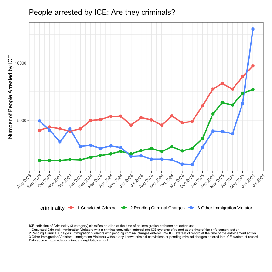
This data visualization makes salient that in recent months, there has been an increase in the number of people arrested (since January 2025), though the most pronounced increases have been with “Other Immigration Violators”, defined by ICE as “Immigration Violators without any known criminal convictions or pending criminal charges entered into ICE system of record.”
How are the people arrested by ICE being apprehended?
Now let’s break down these trends by apprehension method. First, we need
to determine what apprehension methods are annotated in this dataset. We
can use table the count the instance of each apprehension method.
methods <- sort(table(arrests_df$method), decreasing=TRUE)
head(methods)
##
##   CAP Local Incarceration      Non-Custodial Arrest                   Located
##                    113134                     57497                     31929
## CAP Federal Incarceration   CAP State Incarceration    ERO Reprocessed Arrest
##                     23580                     10463                      9135
Based on this, from Sep. 2023 to Late Jul. 2025, 120570 arrests have been made via “CAP Local Incarceration”, whereas 64568 have been made via “Non-Custodial Arrest”, 35898 via the “Located” method, and so forth.
“CAP Local Incarceration” refers to the CAP (Criminal Alien Program), an ICE program that targets undocumented immigrants with criminal records for deportation. CAP Local Incarceration refers ICE officers identifying, screening, and interviewing incarcerated individuals in local jails to find allegedly deportable noncitizens for removal proceedings.
We can focus on only the individuals arrested via the CAP Local
Incarceration apprehension method using the filter function and repeat
our previous procedure to make a data visualization of criminality of
people arrested by ICE over time.
mm <- "CAP Local Incarceration"

arrests_df_summary_sub <- arrests_df %>%
  filter(method == mm) %>%
  mutate(month = as.Date(floor_date(date, unit = "month"))) %>%
  group_by(month, criminality) %>%
  summarise(count = n(), .groups = 'drop')

p1 <- ggplot(arrests_df_summary_sub, aes(x = month, y = count, group = criminality, color = criminality)) +
  geom_line(lwd=1.5) +
  geom_point(size=3) +
  scale_x_date(date_breaks = "1 month", date_labels = "%b %Y") +
  labs(
    title = "People arrested by ICE: Are they criminals?",
    subtitle = paste0("Criminality of people arrested by ICE using the ", mm, " method"),
    caption = "CAP Local Incarceration refers to the Criminal Alien Program where ICE officers identify incarcerated individuals in local jails for removal.

ICE definition of Criminality (3-category) classifies an alien at the time of an immigration enforcement action as:
1 Convicted Criminal: Immigration Violators with a criminal conviction entered into ICE systems of record at the time of the enforcement action.
2 Pending Criminal Charges: Immigration Violators with pending criminal charges entered into ICE system of record at the time of the enforcement action.
3 Other Immigration Violators: Immigration Violators without any known criminal convictions or pending criminal charges entered into ICE system of record.
Data source: https://deportationdata.org/data/ice.html",
    x = "",
    y = "Number of People Arrested by ICE"
  ) +
  theme_bw(base_size = 13) +
  theme(
    plot.title = element_text(size = 18, lineheight = 1.9, vjust = 3),
    axis.title = element_text(size = 13),
    axis.text = element_text(size = 10),
    plot.subtitle = element_text(size = 13, lineheight = 0.9),
    plot.caption = element_text(size = 8, vjust = -10, hjust = 0),
    legend.position = "bottom",
    axis.text.x = element_text(angle = 45, hjust = 1),
    plot.margin = margin(t = 30, r = 20, b = 90, l = 20)
  )
print(p1)
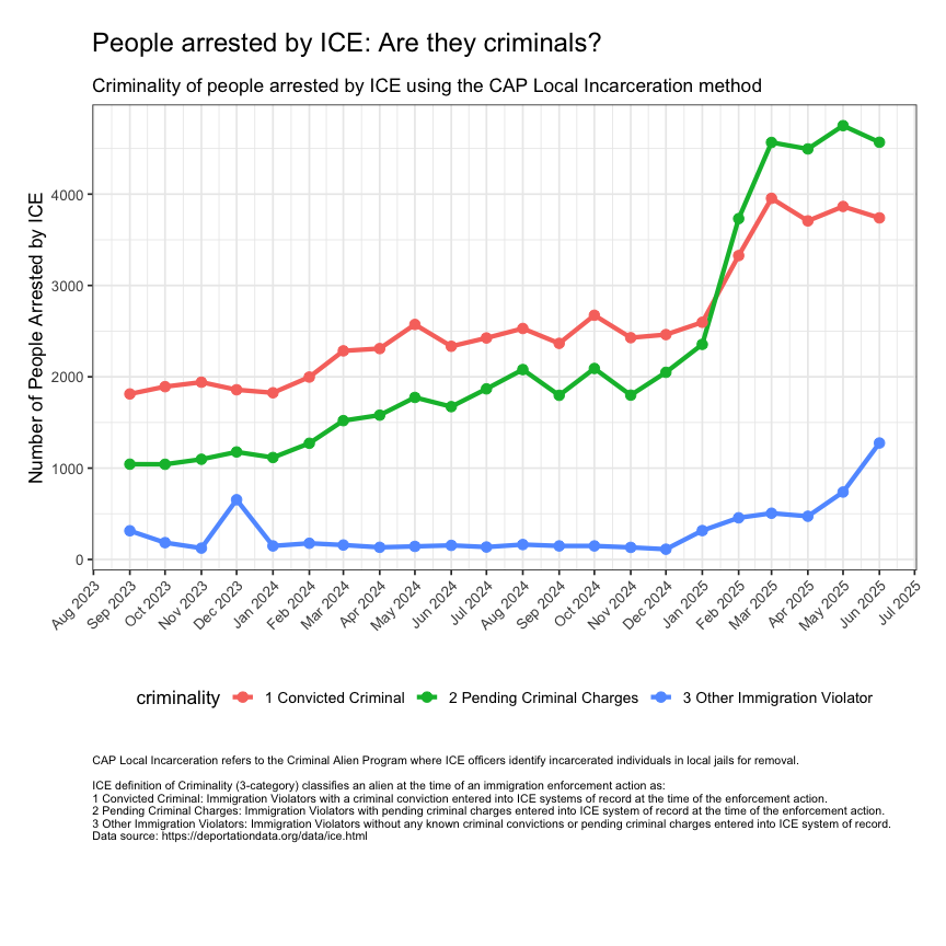
This data visualization makes salient that via the CAP Local Incarceration apprehension method, there has been an increase in the number of “Convicted Criminals” and individuals with “Pending Criminal Charges” arrested by ICE in recent months.
Keep in mind these are individuals already incarcerated in local jails, hence it is perhaps unsurprising that they would also meet the definition of “Convicted Criminal: Immigration Violators with a criminal conviction entered into ICE systems of record at the time of the enforcement action” or “Pending Criminal Charges: Immigration Violators with pending criminal charges entered into ICE system of record at the time of the enforcement action.”
But what about the 35898 people who have been “Located”? This apprehension method refers to ICE arresting undocumented immigrants in the community rather than in a custodial setting, such as a jail or prison.
We can simply update our code to filter by a different apprehension method and visualize the results.
mm <- "Located"

arrests_df_summary_sub <- arrests_df %>%
  filter(method == mm) %>%
  mutate(month = as.Date(floor_date(date, unit = "month"))) %>%
  group_by(month, criminality) %>%
  summarise(count = n(), .groups = 'drop')

p2 <- ggplot(arrests_df_summary_sub, aes(x = month, y = count, group = criminality, color = criminality)) +
  geom_line(lwd=1.5) +
  geom_point(size=3) +
  scale_x_date(date_breaks = "1 month", date_labels = "%b %Y") +
  labs(
    title = "People arrested by ICE: Are they criminals?",
    subtitle = paste0("Criminality of people arrested by ICE using the ", mm, " method"),
    caption = "The Located apprehension method refers to ICE arresting people in the community rather than in a custodial setting, such as a jail or prison.

ICE definition of Criminality (3-category) classifies an alien at the time of an immigration enforcement action as:
1 Convicted Criminal: Immigration Violators with a criminal conviction entered into ICE systems of record at the time of the enforcement action.
2 Pending Criminal Charges: Immigration Violators with pending criminal charges entered into ICE system of record at the time of the enforcement action.
3 Other Immigration Violators: Immigration Violators without any known criminal convictions or pending criminal charges entered into ICE system of record.
Data source: https://deportationdata.org/data/ice.html",
    x = "",
    y = "Number of People Arrested by ICE"
  ) +
  theme_bw(base_size = 13) +
  theme(
    plot.title = element_text(size = 18, lineheight = 1.9, vjust = 3),
    axis.title = element_text(size = 13),
    axis.text = element_text(size = 10),
    plot.subtitle = element_text(size = 13, lineheight = 0.9),
    plot.caption = element_text(size = 8, vjust = -10, hjust = 0),
    legend.position = "bottom",
    axis.text.x = element_text(angle = 45, hjust = 1),
    plot.margin = margin(t = 30, r = 20, b = 90, l = 20)
  )
print(p2)
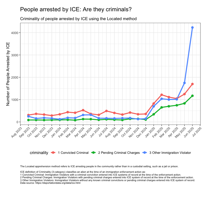
This data visualization makes salient that via the Located apprehension method, while there was a slight increase in the number of arrests across all criminality categories after January 2025, since April 2025, there has been an drastic increase in the number of “Other Immigration Violators: Immigration Violators without any known criminal convictions or pending criminal charges entered into ICE system of record” arrested by ICE.
We can also use gganimate to make an animated version of this data visualization
to emphasize the change over time.
library(gganimate)
# Animate
panim <- p2 +
  transition_reveal(along = month) +
  enter_fade() +
  exit_fade() +
  view_follow(fixed_y = FALSE)

# Render
animate(panim,
        width = 800,
        height = 800,
        fps = 20,
        duration = 10,
        end_pause = 100)
Who is being located and arrested by ICE?
Because this data provides information on individuals, we can in theory
cross reference news and other information to determine who specifically
is being located in the community and arrested by ICE. Let’s go back to
our original arrests table.
I am interested in focusing on people who were arrested via the “Located” apprehension method, who are not criminals (so “3 Other Immigration Violator”), who were arrested recently (after July), and let’s say in the state of Oregon. We can design a set of filters based on these criteria.
findperson <- arrests %>%
  filter(apprehension_method == "Located") %>%
  filter(apprehension_criminality == "3 Other Immigration Violator") %>%
  filter(apprehension_date > as.Date("2025-07-01")) %>%
  filter(apprehension_state == 'OREGON')

print(findperson)
## # A tibble: 15 × 23
##    apprehension_date   apprehension_state apprehension_aor         final_program
##    <dttm>              <chr>              <chr>                    <chr>
##  1 2025-07-08 00:00:00 OREGON             Seattle Area of Respons… Non-Detained…
##  2 2025-07-08 00:00:00 OREGON             Seattle Area of Respons… Non-Detained…
##  3 2025-07-09 00:00:00 OREGON             Seattle Area of Respons… Fugitive Ope…
##  4 2025-07-09 00:00:00 OREGON             Seattle Area of Respons… Fugitive Ope…
##  5 2025-07-09 00:00:00 OREGON             Seattle Area of Respons… Fugitive Ope…
##  6 2025-07-09 00:00:00 OREGON             Seattle Area of Respons… Non-Detained…
##  7 2025-07-11 00:00:00 OREGON             Seattle Area of Respons… Fugitive Ope…
##  8 2025-07-15 00:00:00 OREGON             Seattle Area of Respons… ERO Criminal…
##  9 2025-07-15 00:00:00 OREGON             Seattle Area of Respons… Fugitive Ope…
## 10 2025-07-16 00:00:00 OREGON             Seattle Area of Respons… Fugitive Ope…
## 11 2025-07-16 00:00:00 OREGON             Seattle Area of Respons… Fugitive Ope…
## 12 2025-07-23 00:00:00 OREGON             Seattle Area of Respons… Fugitive Ope…
## 13 2025-07-23 00:00:00 OREGON             Seattle Area of Respons… Non-Detained…
## 14 2025-07-23 00:00:00 OREGON             Seattle Area of Respons… Non-Detained…
## 15 2025-07-23 00:00:00 OREGON             Seattle Area of Respons… Non-Detained…
## # ℹ 19 more variables: final_program_group <chr>, apprehension_method <chr>,
## #   apprehension_criminality <chr>, case_status <chr>, case_category <chr>,
## #   departed_date <dttm>, departure_country <chr>, final_order_yes_no <chr>,
## #   final_order_date <dttm>, birth_year <dbl>, citizenship_country <chr>,
## #   gender <chr>, apprehension_site_landmark <chr>, unique_identifier <chr>,
## #   apprehension_date_time <dttm>, duplicate_likely <lgl>, file_original <chr>,
## #   sheet_original <chr>, row_original <dbl>
There are 15 people meeting such a criteria. Of these people, we can see on July 15th, a 38-year-old (born 1987) man from Iran was located and arrested by ICE.
print(data.frame(findperson[8,]))
##   apprehension_date apprehension_state               apprehension_aor
## 1        2025-07-15             OREGON Seattle Area of Responsibility
##                final_program final_program_group apprehension_method
## 1 ERO Criminal Alien Program                 ICE             Located
##       apprehension_criminality case_status
## 1 3 Other Immigration Violator      ACTIVE
##                                               case_category departed_date
## 1 [8B] Excludable / Inadmissible - Under Adjudication by IJ          <NA>
##   departure_country final_order_yes_no final_order_date birth_year
## 1              <NA>                 NO             <NA>       1987
##   citizenship_country gender                 apprehension_site_landmark
## 1                IRAN   Male PORTLAND FUGITIVE OPERATIONS STREET ARREST
##                          unique_identifier apprehension_date_time
## 1 452684b1b9e6273464e420ab79051f6c563180ff    2025-07-15 10:33:32
##   duplicate_likely
## 1            FALSE
##                                                                    file_original
## 1 2025-ICLI-00019_2024-ICFO-39357_ERO Admin Arrests_LESA-STU_FINAL Redacted.xlsx
##   sheet_original row_original
## 1  Admin Arrests        77728
Cross-referencing news media, I believe this arrest entry to correspond to Mahdi Khanbabazadeh, a 38 man born in Iran and married to a U.S. citizen, who was located by ICE and arrested while he was driving his child to Guidepost Montessori school in South Beaverton Oregon on July 15.
As such, cross-referencing multiple information sources using such individual-level data has allowed us to identify a concrete, individual example of a person being detained by ICE using the “Located” apprehension method.
Thoughts and conclusions
We have performed an exploratory data analysis via data visualization of publicly available ICE arrests data from the The Deportation Data Project. As with any exploratory data analysis, be they for biomedical data or ICE arrest data, the results allow us to form a working hypothesis that we can then iterate on with additional data collection and analyses. It will be left up as an exercise to the student to form these hypotheses for themselves.
See if you can integrate this dataset with our previous ICE detention dataset to explore additional questions and visualize additional trends.
Try it out for yourself!
Try and take a look at the data for yourself. See what additional hypotheses you may be able to generate from exploring these datasets.
Some questions to explore include:
- Repeat this analysis filtering the data to focus on your local community by state.
- What time of day are ICE locating individuals? Are there any trends in
apprehension_time? - Where are ICE locating individuals? Use what you learned from our previous post to explore geographical trends.
Recent Posts
- The Mentorship Index on 01 March 2026
- Vibe coding with SEraster and STcompare to compare spatial transcriptomics technologies on 22 February 2026
- RNA velocity in situ infers gene expression dynamics using spatial transcriptomics data on 13 October 2025
- Analyzing ICE Arrest Data - Part 2 on 27 September 2025
- Analyzing ICE Detention Data from 2021 to 2025 on 10 July 2025
Related Posts
- Analyzing ICE Detention Data from 2021 to 2025
- Multi-sample Integrative Analysis of Spatial Transcriptomics Data using Sketching and Harmony in Seurat
- Using AI to find heterogeneous scientific speakers
- The many ways to calculate Moran's I for identifying spatially variable genes in spatial transcriptomics data